Fundamentals of Linear Array Processing – Receive Beamforming

In the previous two posts we discussed the fundamentals of array processing particularly the concept of beamforming (please check out array processing Part-1 and Part-2). Now we build upon these concepts to introduce some linear estimation techniques that are used in array processing. These are particularly suited to a situation where multiple users are spatially distributed in a cell and they need to be separated based upon their angles of arrival. But first let us introduce the linear model; I am sure you have seen this before.

x=Hs+w

Here, s is the vector of symbols transmitted by M users, H is the N x M channel matrix, w is the noise vector of length N and x is the observation vector of length N. The channel matrix formed by the channel coefficients is deterministic (as opposed to probabilistic) in nature as it is purely dependent upon the phase shifts that the channel introduces due to varying path lengths between the transmit and receive antennas. The impact of a channel coefficient can be thought of as a rotation of the complex signal without altering its amplitude.

This means that the channel acts like a single tap filter and the process of convolution is reduced to simple multiplication (a reasonable assumption if the symbol length is much larger than the channel delay spread). The channel model does not accommodate for path loss and fading that are also inherent characteristics of the channel. But the techniques are general enough for these effects to be factored in later. Furthermore, it is assumed that the channel H is known at the receiver. This is a realistic assumption if the channel is slowly varying and can be estimated by sending pilot signals.

So going back to the linear model we see that we know x and H while s and w are unknown. Here w cannot be estimated since it’s random in nature (remember what the term AWGN stands for?) and we ignore it for the moment. The structure of s is known. For example if we are using BPSK modulation then the m symbols of the signal vector s can either be +1 or -1. So we can start the process of symbol detection by substituting all possible combinations of s₁, s₂…s_m and determine the combination that minimizes

||x-Hs||

This is called the Maximum Likelihood (ML) solution as it determines the combination that was most likely to have been transmitted based upon the observation.

Although ML is conceptually very appealing and yields good results it becomes prohibitively complex as the constellation size or number of transmit antennas increases. For example for 2-Transmit case and BPSK modulation there are 2^(1 bit x 2 antennas)=2^2=4 combinations, which seems quite simplistic. But if 16-QAM modulation is used and there are 4-Transmit antennas the number of combinations increases to 2^(4 bits x 4 antennas)=2^16=65536. So we conclude that ML is not the solution we are looking for if computational complexity is an issue (which might become less of an issue as the processing power of devices increases).

Next we turn our attention to a technique popularly known as Zero Forcing or ZF (the origins of the name I still do not know). According to this technique the channel has a multiplicative effect on the signal. So to remove this effect we simply divide the signal by the channel or in the language of matrices we perform matrix inversion. Mathematically we have:

x=Hs+w

H^-1x=H^-1Hs+H^-1w

H^-1x=s+H^-1w=s̄

So we see that we get back the signal s but we also get a noise component enhanced by inverse of the channel matrix. This is the well-known problem of ZF called Noise Enhancement. Then there are other problems such as non-existence of the inverse when the channel H is not a square matrix (which only happens when the number of transmit and receive antennas is the same). The inverse of H also cannot be calculated if H is not full rank or determinant of H is zero.  So we now introduce another technique called Least Squares (LS). According to this the signal vector can be estimated as

s̄=(H^HH)^-1H^Hx

This is also sometimes referred to as the Minimum Variance Unbiased Estimator, as described by Steven M. Kay in his classical book on Estimation Theory [Fundamentals of Statistical Signal Processing Vol-1]. This can be easily implemented in MATLAB using Moore Penrose Pseudo Inverse or pinv(H). This is much more stable than going for the direct inversion methods.

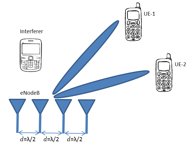
We next plot the Bit Error Rate (BER) using the code below. The number of receive antennas is varied from two to ten while the number of transmit antennas is fixed at four. The transmit antennas are assumed to be positioned at 30, 40, 50 and 60 degrees from the axis of the receive array. The receive antennas are separated by λ/2 meters. The frequency of operation is 1GHz but it is quite irrelevant to the scenario considered as everything is measured in multiples of wavelengths. The Eb/No ratio (roughly the signal to noise ratio) is varied from 5dB to 20dB in steps of 5dB.

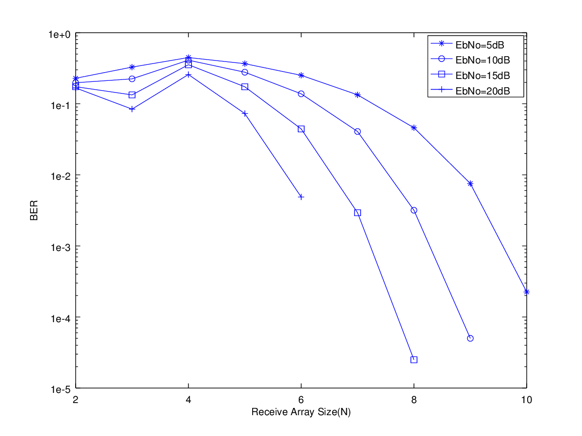
As expected the BER for the two methods, other than ML, is more or less the same and decreases rapidly once the number of receive antennas becomes greater than number of transmit antennas (or number of signals).  The case where the number of receive antennas is less than number of signals (equal powered and with a small angular separation) is dealt with by Overloaded Array Processing (OLAP) techniques and have been discussed in detail by James Hicks [Doctoral Dissertation] a student of Dr. Reed at Virginia Tech.

Strangely enough it is seen that the overloaded case is not the worst part of the BER curve. The worst BER is observed when the number the number of transmit and receive antennas is the same (four in this case). In other words the BER gradually increases as the rank of the channel matrix increases and then decreases once it reaches its maximum value. This is quite interesting and obviously has to do with Noise Enhancement that we discussed earlier. This will be further investigated in future posts.

For further information on the above methods visit this interesting article.

Update-1

So we struggled for a while to find out why the BER is worst at full rank and thought that there is something wrong in our model but ultimately we found that this has to do with how the pseudoinverse works and the way the tolerance limit (tol in MATLAB) for the singular values is set. We have found quite interesting results while experimenting with various inversion methods and the results are pending publication. Will keep you updated about the progress.

Update-2

We experimented with the MATLAB function pinv by changing the tolerance parameter. Previously we had used the default tolerance that is built into the function pinv. The default tolerance (tol) is defined as:

tol = max (size (H)) * sigma_max (H) * eps

where sigma_max (H) is the maximal singular value of channel matrix H

and eps is the machine precision.

More precisely, eps is the relative spacing between any two adjacent numbers in the machine’s floating point system. This number is obviously system dependent. On machines that support IEEE floating point arithmetic, eps is approximately 2.2204e-16 for double precision and 1.1921e-07 for single precision.

So back to the subject we experimented with two values of tol; 1.0 and 0.1 while changing the signal to noise ratio. The number of transmit antennas (users) is fixed at 4 while number of receive antennas is varied from 2 to 8. For tol value of 1.0 it is seen that changing the value of EbNo does not change the results much up to 6 receive antennas but after that the BER results rapidly diverge. For tol value of 0.1 the results are quite unexpected. The BER drops with increasing number of antennas up to N=5 but then there is an unexpected increase in the BER for N=6. This needs to be further investigated.

MATLAB CODE USED TO GENERATE ABOVE PLOT

%%%%%%%%%%%%%%%%%%%%%%%%%%%%%%%%%%%%
% MULTIUSER DETECTION USING 
% A UNIFORM LINEAR ARRRAY
% AKA RECEIVE BEAMFORMING
% COPYRIGHT RAYMAPS (C) 2018
%%%%%%%%%%%%%%%%%%%%%%%%%%%%%%%%%%%%

clear all
close all

% SETTING THE PARAMETERS FOR THE SIMULATION
f=1e9;        %Carrier frequency
c=3e8;        %Speed of light
l=c/f;        %Wavelength
d=l/2;        %Rx array spacing
N=10;         %Receive array length

theta=([30 40 50 60])*pi/180;   %Angular placement of Tx array (users)
EbNo=10;                        %Energy per bit to noise PSD
sigma=1/sqrt(2*EbNo);           %Standard deviation of noise

n=1:N;                          %Rx array vector
n=transpose(n);                 %Converting row to column
M=length(theta);                %Tx array length 

% RECEIVE SIGNAL MODEL (LINEAR)
s=2*(round(rand(M,1))-0.5);           %BPSK signal of length M
H=exp(-i*(n-1)*2*pi*d*cos(theta)/l);  %Channel matrix of size NxM
wn=sigma*(randn(N,1)+i*randn(N,1));   %AWGN noise of length N
x=H*s+wn;                             %Receive vector of length N

% PINV without tol
% y=pinv(H)*x;

% PINV with tol
y=pinv(H, 0.1)*x;

% DEMODULATION AND BER CALCULATION
s_est=sign(real(y));          %Demodulation
ber=sum(s!=s_est)/length(s);  %BER calculation