In a previous post we had discussed MIMO capacity in a fading environment and compared it to AWGN capacity. It sometimes feels unintuitive that fading capacity can be higher than AWGN capacity. If a signal is continuously fluctuating how is it possible that we are able to have reliable communication. But this is the remarkable feature of MIMO systems that they are able to achieve blazing speeds over an unreliable channel, at least theoretically. It has been shown mathematically that an NxN MIMO channel is equivalent to N SISO channels in parallel.

In this post we consider three types of multiple antenna systems namely; MIMO, SIMO and MISO. SISO we will ignore here as it has been discussed in a number of posts. We will present the mathematical framework used to calcualte capacity in each of the three cases and give simulation results. We will compare fading capacity with AWGN capacity and discuss the distinct behavior in the above mentioned three cases. One point to be noted here is that capacity discussed here is ergodic capacity, where it is assumed that the channel transitions over all the fading states.

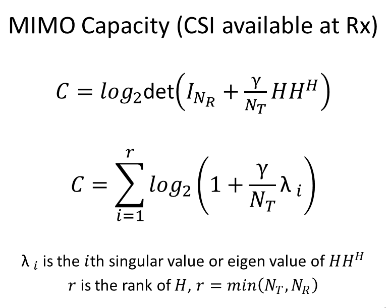
MIMO Capacity

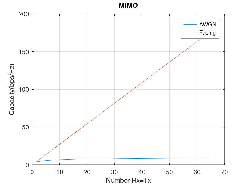
The capacity gains in a spatially uncorrelated MIMO fading channel are the highest. There is no comparison with an AWGN channel which lags far behind. As mentioned previously an NxN MIMO channel is equivalent to N parallel SISO channels i.e. there is a linear increase in capacity with increase in number of Tx and Rx antennas. Mathematically, the reason behind this is that an NxN channel matrix H as defined here is full rank, where rank is min(Nt,Nr). When Nt or Nr decreases the rank decreases and consequentially capacity decreases. Capacity is also impacted if there is correlation between antennas at Tx or Rx.

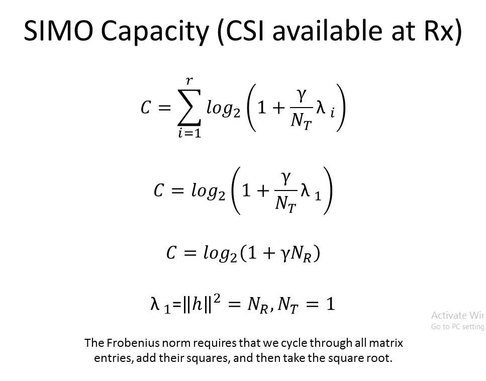
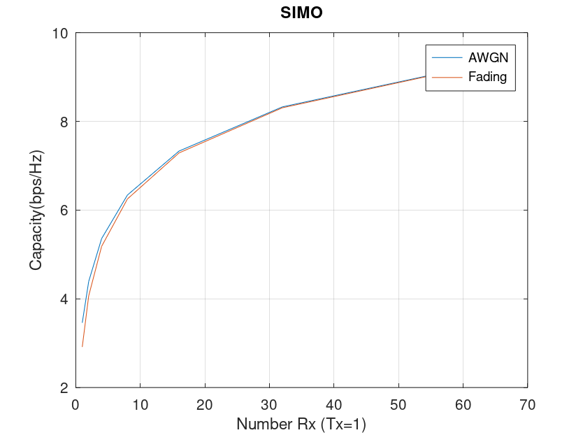
SIMO Capacity

A SIMO channel is one where there is only a single transmit antenna and Nr receive antennas. There is no capacity advantage in a fading environment over an AWGN environment in this case. The main reason is that the channel is known at the receiver so there is no difference between a faded signal and an unfaded signal after equalization has been performed. In both the scenarios the capacity increase with increase in Nr is not linear, rather it is logarithmic. It can also be explained by the fact that the rank of H is one so there is no multiplexing gain in this case. The capacity improvement is due to increase in SNR.

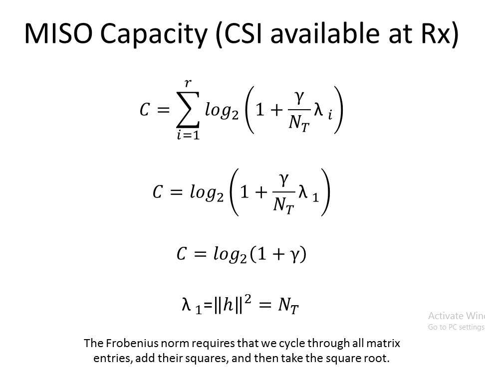
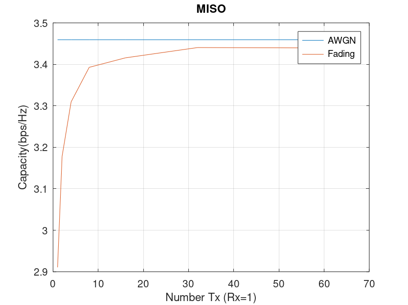
MISO Capacity

A MISO channel is one where there are multiple transmit antennas and single receive antenna. This is the worst type of channel, for the case when CSI is not known at the transmitter. Here the fading capacity is in fact lower than AWGN capacity. But it approaches AWGN capacity as the number of antennas at the transmitter increases. The capacity is in fact equal to SISO channel capcity in an AWGN environment and does not change with number of transmit antennas after a certain threshold is reached. It must be noted that the total transmit power in all the the three cases above is the same.

MATLAB Code

clear all
close all

Nr=16;
Nt=16;
I=eye(Nr);
g=10;

H=ones(Nr,Nt);
C_AWGN=log2(det(I+(g/Nt)*(H*H')));

for n=1:10000
    H=sqrt(1/2)*randn(Nr,Nt)+i*sqrt(1/2)*randn(Nr,Nt);
    C1(n)=log2(det(I+(g/Nt)*(H*H')));
    C2(n)=sum(log2(1+(g/Nt)*(eig(H*H'))));
end
Erg_C_fad1=mean(C1);
Erg_C_fad2=mean(C2);

Note:

1. We have assumed that Channel State Information (CSI) is available at the receiver only. Having CSI at transmitter is desirable but slightly more complicated to estimate.
2. I is an identity matrix, γ is the Signal to Noise Ratio (SNR) and Nt and Nr is the number of transmit and receive antennas respectively.
3. H is an Nr x Nt channel matrix whose entries are complex numbers with IID real and imaginary parts. Both the real and imaginary parts have Gaussian distribution with a mean of zero and variance 0.5 resulting in an amplitude which is Rayleigh distributed and a phase which is uniformly distributed. This is referred to as a flat fading channel.

Reference:

Rafik Ahmad, Devesh Pratap Singh, Mitali Singh, “Ergodic Capacity of MIMO Channel in Multipath Fading Environment,” I.J. Information Engineering and Electronic Business, 2013, 3, 41-48.
https://www.mecs-press.org/ijieeb/ijieeb-v5-n3/IJIEEB-V5-N3-5.pdf

Author: Yasir Ahmed (aka John)

More than 20 years of experience in various organizations in Pakistan, the USA, and Europe. Worked as a Research Assistant within the Mobile and Portable Radio Group (MPRG) of Virginia Tech and was one of the first researchers to propose Space Time Block Codes for eight transmit antennas. The collaboration with MPRG continued even after graduating with an MSEE degree and has resulted in 12 research publications and a book on Wireless Communications. Worked for Qualcomm USA as an Engineer with the key role of performance and conformance testing of UMTS modems. Qualcomm is the inventor of CDMA technology and owns patents critical to the 4G and 5G standards.

Twitter Facebook Linkedin