Fundamentals of Direction of Arrival Estimation

Direction of Arrival (DOA) estimation is a fundamental problem in communications and signal processing with application in cellular communications, radar, sonar etc. It has become increasingly important in recent times as 5G communications uses DOA to spatially separate the users resulting in higher capacity and throughput. Direction of Arrival estimation can be thought of as the converse of beamforming. As you might recall from the discussion in previous posts, in beamforming you use the steering vector to receive a signal from a particular direction, rejecting the signals from other directions. In DOA estimation you scan the entire angular domain to find the required signal or signals and estimate their angles of arrival and possibly the ranges as well.

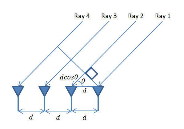
The theory of DOA estimation draws from the techniques and algorithms used for spectral estimation, as finding the angle of arrival in the spatial domain is the same as finding the frequency of a windowed signal in the temporal domain. Just as we have to follow the Nyquist’s sampling theorem in time domain, we have to follow the spatial sampling theorem when implementing beamforming or DOA estimation. Some of the popular techniques used for DOA estimation are correlation, MVDR, FFT, MUSIC and ESPRIT. We only discuss the first two in this section as the remaining ones are discussed in detail in the posts on phase and frequency.

Correlation or Delay and Sum (DS) method, as it is sometimes referred to, is the simplest and most effective technique and works quite well at low SNRs and with moderate array size. Minimum Variance Distortionless Response (MVDR) on the other hand is a bit more complicated as it requires estimation of the correlation matrix and also requires couple of matrix inversions. As you may already know matrix inversion is a tricky subject and if the matrix is ill conditioned the inverse may not even exist. A technique usually used to get around this problem is to use the Moore Penrose Pseudo Inverse instead of direction inversion. Another problem with MVDR is that for estimating the correlation matrix you need multiple snapshots to get good results.   

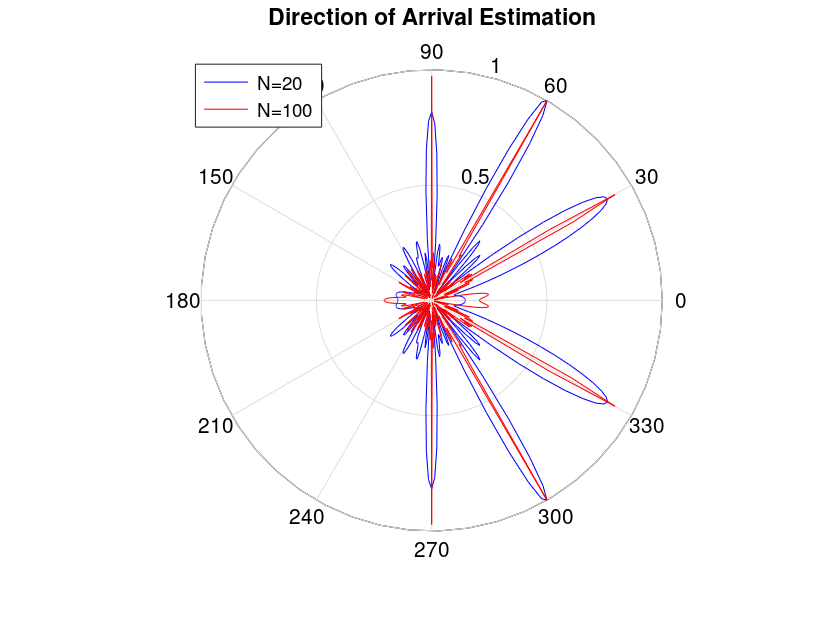
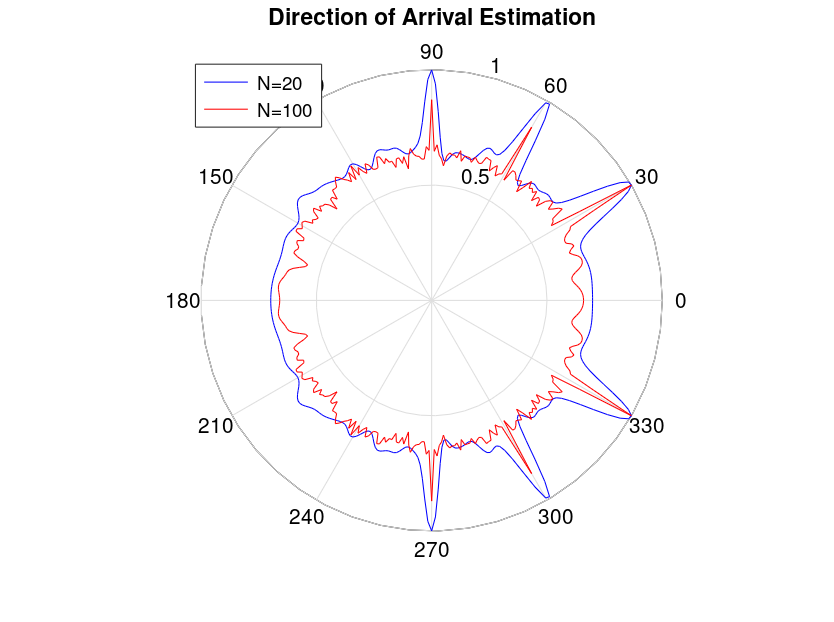
Given below is the code and simulation results for both the techniques. We have assumed a frequency of 1GHz, antenna spacing of λ/2, angles of arrival of 30, 60 and 90 degrees, signal to noise ratio of 0dB (per element) and scan resolution of 1 degree over azimuth. Antenna array size is varied from 20 elements to 100 elements and correlation matrix for MVDR is calculated using 1000 snapshots (no averaging is used for DS). It is seen that performance of simple correlation scheme is quite respectable even for a receive array size of 20 and improves appreciably when the array size is increased to 100 (pencil beam is obtained). This is not the case for MVDR which is highly sensitive to noise level and performance is not that great even for N=100. However, a surprising result was that MVDR performs better than DS in very poor SNR (which can be attributed to averaging used in calculation of correlation matrix for MVDR).

Mathematically the two methods can be described as:

Code for Direction of Arrival Estimation Using Correlation Method

%%%%%%%%%%%%%%%%%%%%%%%%%%%%%%%%%%%%%%%%%%%%%
% DIRECTION OF ARRIVAL ESTIMATION USING A ULA
% CORRELATION METHOD
% N is the number of elements
% d is the inter-element spacing
% theta is the angle of arrival
% Copyright 2022 RAYmaps
%%%%%%%%%%%%%%%%%%%%%%%%%%%%%%%%%%%%%%%%%%%%%
clear all
close all

f=1e9;
c=3e8;
l=c/f;
d=l/2;
N=20;
phi=0:pi/180:2*pi;

theta1=pi/6;
theta2=pi/3;
theta3=pi/2;
n=1:N;
n=transpose(n);

x1=exp(-i*(n-1)*2*pi*d*cos(theta1)/l);
x2=exp(-i*(n-1)*2*pi*d*cos(theta2)/l);
x3=exp(-i*(n-1)*2*pi*d*cos(theta3)/l);

x=x1+x2+x3;
y=x+0.7071*(randn(N,1)+i*randn(N,1));
w=exp(-i*(n-1)*2*pi*d*cos(phi)/l);
r=w'*y;

polar(phi,abs(r)/max(abs(r)),'b')
title ('Direction of Arrival Estimation')
%%%%%%%%%%%%%%%%%%%%%%%%%%%%%%%%%%%%%%%%%%%%%

Code for Direction of Arrival Estimation Using MVDR Method

%%%%%%%%%%%%%%%%%%%%%%%%%%%%%%%%%%%%%%%%%%%%%
% DIRECTION OF ARRIVAL ESTIMATION USING A ULA
% MVDR METHOD
% N is the number of elements
% d is the inter-element spacing
% theta is the angle of arrival
% Copyright 2022 RAYmaps
%%%%%%%%%%%%%%%%%%%%%%%%%%%%%%%%%%%%%%%%%%%%%
clear all
close all

f=1e9;
c=3e8;
l=c/f;
d=l/2;
N=20;
phi=0:pi/180:2*pi;
theta=[pi/6, pi/3, pi/2];
n=transpose(1:N);

x1=exp(-i*(n-1)*2*pi*d*cos(theta(1))/l);
x2=exp(-i*(n-1)*2*pi*d*cos(theta(2))/l);
x3=exp(-i*(n-1)*2*pi*d*cos(theta(3))/l);
x=x1+x2+x3;
R=zeros(N,N);

for m=1:1000
   y=x+0.7071*(randn(N,1)+i*randn(N,1));
   R=R+y*y';
end

R=R/m;
R1=pinv(R,0.1);
w=exp(-i*(n-1)*2*pi*d*cos(phi)/l);

for k=1:length(phi);
   w1=w(:,k);
   P(k)=abs(pinv(w1'*R1*w1,0.1));
end

polar(phi,P/max(P),'b')
title ('Direction of Arrival Estimation')
%%%%%%%%%%%%%%%%%%%%%%%%%%%%%%%%%%%%%%%%%%%%%

Note:

1. Please
   note that so far our analysis is based on visual inspection, which can be
   misleading. It is possible that a particular technique may have smaller peaks
   but accuracy of angular information is greater. For more in depth analysis we
   need to compare the Mean Square Error (MSE) to Cramer Rao Lower Bound (CRLB).
   We also need to decrease the step size for the scan.
2. Please
   note that we have scanned the entire angular domain from 0 to 360 degrees to
   find the DOA. In ULA theory it is known that response is symmetrical about the
   axis of the array so typically only 0 to 180 degrees is scanned.
3. Some
   interesting antenna patterns can be obtained by using non-uniform antenna
   arrays and we hope to discuss this in a future post.
4. Beamforming
   and DOA go hand in hand. DOA finds the angle of arrival and then the
   base-station can form a beam on that angle using beamforming techniques.
5. Minimum
   Variance Distortionless Response is also known Capon estimator after its
   founder J. Capon who proposed his spectral analysis method in 1969.

References

https://www.comm.utoronto.ca/~rsadve/Notes/DOA.pdf

https://arxiv.org/pdf/2002.01588.pdf

https://escholarship.org/content/qt1w13p71p/qt1w13p71p_noSplash_9f69e592ae9b76ba11f4349daa613333.pdf

Author: Yasir

More than 20 years of experience in various organizations in Pakistan, the USA, and Europe. Worked with the Mobile and Portable Radio Group (MPRG) of Virginia Tech and Qualcomm USA and was one of the first researchers to propose Space Time Block Codes for eight transmit antennas. Have publsihed a book “Recipes for Communication and Signal Processing” through Springer Nature.

Twitter Facebook Linkedin