In the previous post we had discussed the fundamentals of a Uniform Linear Array (ULA). We had seen that as the number of array elements increases the Gain or Directivity of the array increases. We also discussed the Half Power Beam Width (HPBW) that can be approximated as 0.89×2/N radians. This is quite an accurate estimate provided that the number of array elements ‘N’ is sufficiently large.
But the max Gain is always in a direction perpendicular to the array. What if we want the array to have a high Gain in another direction such as 45 degrees. How can we achieve this? This has application in Radars where you want to search for a target by scanning over 360 degrees or in mobile communications where you want to send a signal to a particular user without causing interference to other users. One simple way is to physically rotate the antenna but that is not always a feasible solution.
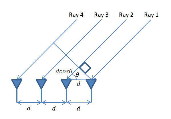
Going back to the basics remember that the Electric field pattern depends upon the constructive and destructive interference of incoming waves. If we have a vector (usually called the steering vector) that aligns the rays coming in from a particular direction we would get a high Gain in that direction. Similarly we can steer a null in a particular direction if we want to reject a particular signal. This we will discuss in a future post.
MATLAB CODE
%%%%%%%%%%%%%%%%%%%%%%%%%%%%%%%%%%%%
% BEAMFORMING USING A
% UNIFORM LINEAR ARRRAY
% COPYRIGHT RAYMAPS (C) 2018
%%%%%%%%%%%%%%%%%%%%%%%%%%%%%%%%%%%%

clear all
close all

f=1e9;
c=3e8;
l=c/f;
d=l/2;
no_elements=10;
phi=pi/6;

theta=0:pi/180:2*pi;
n=1:no_elements;
n=transpose(n);

X=exp(-i*(n-1)*2*pi*d*cos(theta)/l);
w=exp( i*(n-1)*2*pi*d*cos(phi)/l);
w=transpose(w);
r=w*X;

polar(theta,abs(r),'b')
title ('Gain of a Uniform Linear Array')
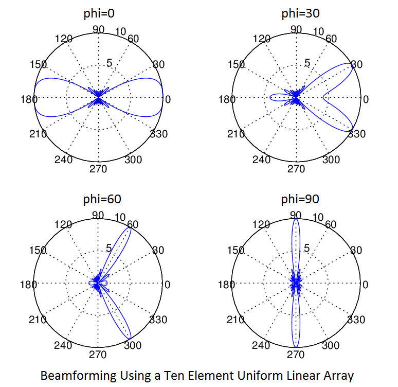
The figure below shows the Electric field pattern of a 10 element array steered towards 0, 30, 60 and 90 degrees respectively. We see that selectivity of the array is higher on the Broadside than on the Endfire. In my opinion this has to do with how the cosine function behaves from 0 to 90 degrees. The rate of change of cosine function is much faster around 90 degrees than at 0 degrees or 180 degrees. The slowly changing cosine in the latter case causes a wide response on the Endfire.
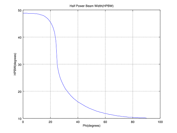
We did calculate the HPBW for a range of steering angles and found that it varied widely from as small as 10.17 degrees to as large as 48.62 degrees. This shows that simple Beamforming using a steering vector has its limitations. The detailed results along with a graph are shown below. It is seen that as the steering angle increases from about 20 degrees there is a sudden decrease in HPBW. For one degree increase of steering angle (phi) from 24 to 25 degrees there is decrease of approx 9 degrees in HPBW. We will investigate this further in future posts.
Case 1: phi = 0, HPBW = 48.62 deg
Case 2: phi = 30, HPBW = 21.69 deg
Case 3: phi = 60, HPBW = 11.75 deg
Case 4: phi = 90, HPBW = 10.17 deg
For further visualization of the variation in antenna pattern as a function of the steering angle please have a look at this Interactive Graph. The parameters that can be varied include the angle of the beam, number of antenna elements and separation of the antenna elements. This is taken from an excellent online resource by the name of Geogebra. For further information on how you can use this tool for your own mathematical problems please do visit their website.
MY FIRST GEOGEBRA VISUALIZATION
Author: Yasir
More than 20 years of experience in various organizations in Pakistan, the USA, and Europe. Worked with the Mobile and Portable Radio Group (MPRG) of Virginia Tech and Qualcomm USA and was one of the first researchers to propose Space Time Block Codes for eight transmit antennas. Have publsihed a book “Recipes for Communication and Signal Processing” through Springer Nature.
14 thoughts on “Basics of Beamforming in Wireless Communications”
Dear John indeed I am learning a lot from your site. But here I am stuck on your answer to Sadaf. As she asked if we want to generate two beams simultaneously in desired directions such as 0 and 30 degrees, then what will we do for that? Your answer is look at Linear Array Processing. Simple techniques like ZF, LS and MMSE can be used to separate users based on their spatial signatures. I looked that too, but I am unable to generate two beams simultaneously. Can you do it foe me here?
Yeah…maybe you do not have visuals to prove it. But try reducing the angular separation between users and see how BER deteriorates.
Dear Sir ,
Why is t=90-phi ?? to calculate the HPBW with this formula
HPBW=(0.886*lambda)/(N*d*cos(t))
Hema,
I did not get your question…can you please elaborate?
YA
Is there any equation between steering angle and HPBW to calculate HPBW or is it measured in the beams plot?
So angle theta is for the formation of the beam, angle phi is for the direction of the beam?
There is an approximate formula for calculation of HPBW and it is given as:
HPBW=(0.886*lambda)/(N*d*cos(t))
where lambda is the wavelength, N is the number of elements, d is the inter-element separation and t is the angle with the normal to the array (or you can say t=90-phi degrees, where phi is the steering angle). However please note that this formula is only accurate for phi close to 90 degrees. For more accurate calculation it is recommended to plot HPBW as a function of the steering angle as shown in above code.
What is the relation between the steering angle and HPBW? Equation?
Thank you ,
If you want to generate two beams simulataneously, targeted at 0 and 30 degrees, how will you do that?
Sadaf,
That’s an excellent question. Please have a look at my posts on Linear Array Processing. Simple techniques like ZF, LS and MMSE can be used to separate users based on their spatial signatures. Thirty degree separation between users is sufficient for a moderate size array at the base station. Users can be separated with much smaller angular separations. Please also have a look at the post on Massive MIMO. Hope this helps.
John
Many thanks for the clarification.