
In the previous post we discussed block codes and their decoding mechanisms. It was observed that with syndrome-based decoding there is only a minimal advantage over the no coding case. With Maximal Likelihood (ML) decoding there is significant improvement in performance but computational complexity increases exponentially with length of the code and alphabet size. This is where convolutional codes come to the rescue.
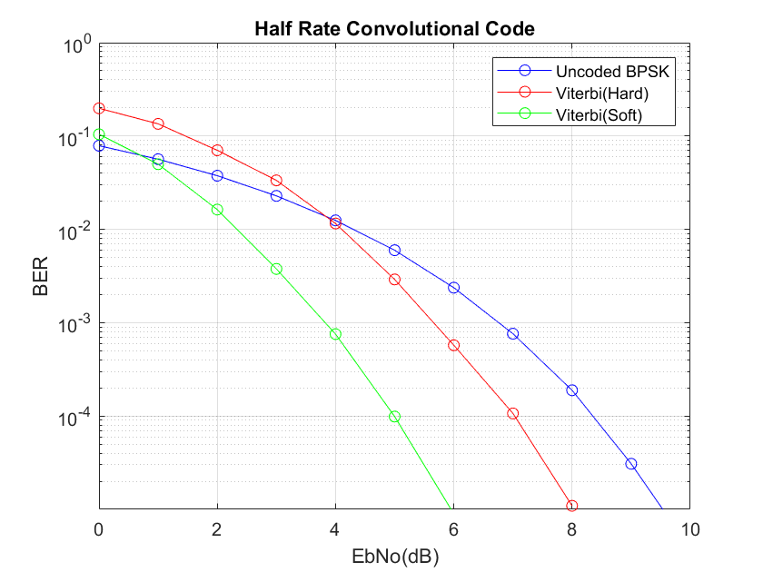
Convolutional codes when decoded using Viterbi Algorithm (VA) provide significant gains over the no coding case. The performance is further improved by using soft metrics instead of hard metrics (Euclidean distance is used in this case instead of Hamming distance). In fact, the performance is even better than brute force ML decoded Hamming (7,4) Code discussed in the previous post.
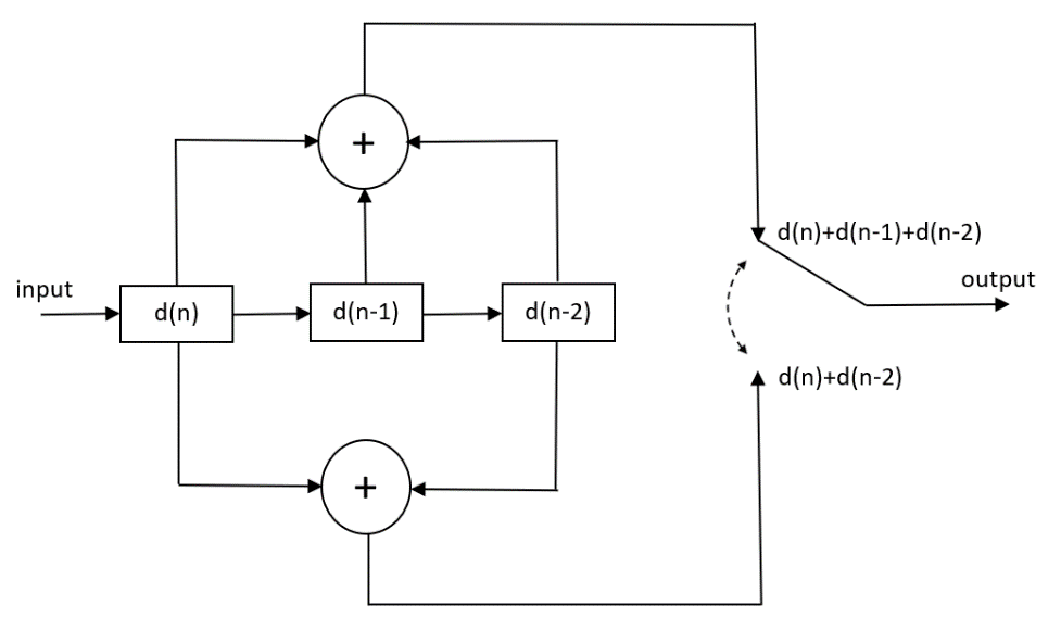
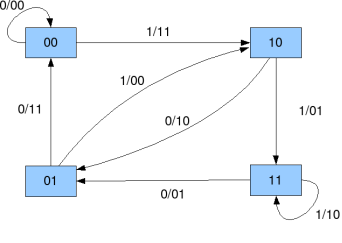
The structure of the convolutional encoder used and state diagram is given below. The constraint length of this code is 3. This is the number of input bits that are used to generate the output bits at any instance of time. Higher the constraint length better is the performance but at the expense of computational complexity. The number of states of the convolutional code is given as 2^(K-1) where K is the constraint length (here K=3 and number of states is 4).
In this example 2 bits are generated at the output for 1 bit at the input resulting in a code rate of ½. This is catered for in the simulation by adjusting the signal to noise ratio so that there is no unfair advantage over the uncoded case. With soft decoding a 2dB performance improvement can be achieved over hard decoding at high signal to noise ratios. Just to be clear, in soft decoding, the distance metric is calculated before a decision is made on which symbol was most likely transmitted based on the observation.
Another important characteristic is the truncation length of the Viterbi Algorithm. This decides how many state transitions are used in the decoding process. Higher the truncation length better is the performance of VA but after a certain point law of diminishing returns sets in. It must be noted that computational complexity of VA is lower than brute force ML decoding that is used for block codes but the performance is much better (at least for the case where soft decoding is used).
%%%%%%%%%%%%%%%%%%%%%%%%%%%%%%%%%%%%%%%%%%%%%%%%%%%%%%%%
% ENCODING AND DECODING OF 1/2 CONVOLUTIONAL CODE
% Number of states is 4
% For each input bit there are 2 output bits
% Constraint length is 3
% Copyright 2020 RAYmaps
%%%%%%%%%%%%%%%%%%%%%%%%%%%%%%%%%%%%%%%%%%%%%%%%%%%%%%%%
clear all
close all

% Encoding and Modulation
ip_length=50000;
msg_bits=round(rand(1,ip_length));
msg_bits=[0,0,msg_bits];
c=[];

for n=1:ip_length
    c1(n)=mod(msg_bits(n)+msg_bits(n+1)+msg_bits(n+2),2);
    c2(n)=mod(msg_bits(n)+msg_bits(n+2),2);
    c=[c,c1(n),c2(n)];
end
cx=2*c-1;

% Noise Addition and Demodulation
Eb=2.0;
EbNo=10.0;
sigma=sqrt(Eb/(2*EbNo));
y=cx+sigma*randn(1,2*ip_length);
d=y>0;

% Path Metric and Branch Metric Calculation
pm1(1)=0;
pm2(1)=1000;
pm3(1)=1000;
pm4(1)=1000;

d=[d,0,0,0,0];
for n=1:ip_length+2
    bm11=sum(abs([d(2*n-1),d(2*n)]-[0,0]));
    bm13=sum(abs([d(2*n-1),d(2*n)]-[1,1]));
    bm21=sum(abs([d(2*n-1),d(2*n)]-[1,1]));
    bm23=sum(abs([d(2*n-1),d(2*n)]-[0,0]));
    bm32=sum(abs([d(2*n-1),d(2*n)]-[1,0]));
    bm34=sum(abs([d(2*n-1),d(2*n)]-[0,1]));
    bm42=sum(abs([d(2*n-1),d(2*n)]-[0,1]));
    bm44=sum(abs([d(2*n-1),d(2*n)]-[1,0]));

    pm1_1=pm1(n)+bm11;
    pm1_2=pm2(n)+bm21;
    pm2_1=pm3(n)+bm32;
    pm2_2=pm4(n)+bm42;
    pm3_1=pm1(n)+bm13;
    pm3_2=pm2(n)+bm23;
    pm4_1=pm3(n)+bm34;
    pm4_2=pm4(n)+bm44;

    if pm1_1<=pm1_2
        pm1(n+1)=pm1_1;
        tb_path(1,n)=0;
    else
        pm1(n+1)=pm1_2;
        tb_path(1,n)=1;
    end

    if pm2_1<=pm2_2
        pm2(n+1)=pm2_1;
        tb_path(2,n)=0;
    else
        pm2(n+1)=pm2_2;
        tb_path(2,n)=1;
    end

    if pm3_1<=pm3_2
        pm3(n+1)=pm3_1;
        tb_path(3,n)=0;
    else
        pm3(n+1)=pm3_2;
        tb_path(3,n)=1;
    end

    if pm4_1<=pm4_2
        pm4(n+1)=pm4_1;
        tb_path(4,n)=0;
    else
        pm4(n+1)=pm4_2;
        tb_path(4,n)=1;
    end
end

[last_pm,last_state]=min([pm1(n+1),pm2(n+1),pm3(n+1),pm4(n+1)]);
m=last_state;

% Traceback and Decoding
for n=ip_length+2:-1:1
    if m==1
        if tb_path(m,n)==0
            op_bits(n)=0;
            m=1;
        elseif tb_path(m,n)==1
            op_bits(n)=0;
            m=2;
        end

    elseif m==2
        if tb_path(m,n)==0
            op_bits(n)=0;
            m=3;
        elseif tb_path(m,n)==1
            op_bits(n)=0;
            m=4;
        end

    elseif m==3
        if tb_path(m,n)==0
            op_bits(n)=1;
            m=1;
        elseif tb_path(m,n)==1
            op_bits(n)=1;
            m=2;
        end

    elseif m==4
        if tb_path(m,n)==0
            op_bits(n)=1;
            m=3;
        elseif tb_path(m,n)==1
            op_bits(n)=1;
            m=4;
        end
    end
end

ber=sum(msg_bits(3:end)~=op_bits(1:end-2))/ip_length
%%%%%%%%%%%%%%%%%%%%%%%%%%%%%%%%%%%%%%%%%%%%%%%%%%%%%%%%
bm: branch metric is the Hamming Distance/Euclidean Distance between the bits/symbols received and bits/symbols corresponding to a certain state transition.
pm: path metric is the total cost of a certain path using Hamming Distance or Euclidean Distance. The path metric for a state is the previous path metric plus the current branch metric that results in the lowest cost to reach this state.
Main Takeaway: A convolutional encoder introduces memory in the bit stream by allowing only certain state transitions and certain outputs at each step. Viterbi decoder makes use of this memory by estimating which sequence of state transitions was most likely to have been made based upon the observations. It breaks down a complex problem into smaller parts, each of one which is quite simple to solve. This is much easier than brute force search that we used in the case of Hamming codes.
Note:
- We have considered BPSK modulation in the simulation above but the code is general enough to accommodate any type of modulation. For complex modulations the Euclidean distance would be calculated in complex domain and AWGN noise added would also be complex.
- It must be noted that for convolutional codes encoding process can be carried out by performing convolutional operation. But we have not used the MATLAB built-in function ‘conv’ for this; rather, we simply perform modulo-2 addition. There is some advantage in using convolution operation, instead of modulo-2 addition, in terms of computation time.
- In the state diagram the rightmost two registers determine the state of the convolutional code. The leftmost register is the input. Together the three bits determine the output at each instant.
- The above code is for hard decision decoding but it can be easily modified for soft decision decoding. EbNo is Energy Per Bit to Noise Power Spectral Density ratio on linear scale.