We have previously discussed Block Codes and Convolutional Codes and their coding and decoding techniques particularly syndrome-based decoding and Viterbi decoding. Now we discuss an advanced form of Block Codes known as Low Density Parity Check (LDPC) codes. These codes were first proposed by Robert Gallager in 1960 but they did not get immediate recognition as they were quite cumbersome to code and decode. But in 1995 the interest in these codes was revived, after discovery of Turbo Codes. Both these codes achieve the Shannon Limit and have been adopted in many wireless communication systems including 5G.
The name LDPC originates from the fact that the parity check matrix of LDPC codes is a sparse matrix with a few ones and lots of zeros e.g., a size 1000 x 2000 parity check matrix might have 3 ones per column and 6 ones per row. This simplifies coding and decoding of LDPC codes. Another point to mention here is that LDPC codes draw their inspiration from Turbo Codes which are iteratively decoded, successively getting closer to the Shannon limit. LDPC codes can be decoded in a number of ways but the most common is serial decoding and parallel decoding, both iterative in nature. We discuss parallel decoding in this post.
If you understand coding and decoding of Block Codes, then half the problem is solved. Let’s consider we have 6 data bits (d1, d2, d3, d4, d5, d6) and 5 parity check bits (p1, p2, p3, p4, p5) that are calculated as per the table below.
| d1 | d2 | d3 | p1 |
| d4 | d5 | d6 | p2 |
| p3 | p4 | p5 |
Structure for Calculating Parity Check Bits
The advantage of such a scheme is that each data bit is protected by multiple parity check bits so the possibility of an error going undetected is reduced. The equations that govern the calculation of parity bits are given below. The bit addition operations are performed modulo-2 (equivalent to XOR operation).
p1=d1⊕d2⊕d3
p2=d4⊕d5⊕d6
p3=d1⊕d4
p4=d2⊕d5
p5=d3⊕d6
It must be noted that during each transmission 6 data bits are transmitted as it is and 5 parity bits are appended to the data bits resulting in a block size of 11. As discussed previously such a code is called systematic code and can easily be encoded and decoded using a generator matrix (G=I|C) and parity check matrix (H=C’|I) respectively. Another important metric of a code is the code rate which governs how much redundancy is added to the uncoded data bits. The code rate in the above example is r=k/n=6/11. Lower the code rate higher is the redundancy and stronger is the code but this is at the expense of spectral efficiency. Typical code rates used in wireless communication systems are 1/3, 1/2, 2/3 etc.
Just as in Block Codes, error detection and correction can be performed by calculating the syndrome but BER performance using this technique is not that great. Maximum Likelihood technique (remember brute search) can be used but it is very computationally complex for large block sizes. Here comes to our rescue a concept from probability theory called Bayes theorem. According to this theorem we can use posterior probabilities to decide which symbol was most likely to have been transmitted. After some simplifications to the Bayes theorem and some more mathematical manipulations we have the following equality.
L(x1 ⊕ x2) = sgn[L(x1)] sgn[L(x2)] min[|L(x1)|, |L(x2)|]
With this equality and parity check equations given above, the extrinsic information of each decoder can be calculated separately (decoder-I operates row wise and decoder-II operates column wise in the above table). This extrinsic information is then used to refine the estimation of the symbol that was most likely to have been transmitted. The sign is used to estimate the transmitted symbol sign and the absolute value provides the information about the reliability of the decoded symbol. As this process is iteratively performed the estimate of the transmitted symbol becomes more and more accurate (we have used up to 25 iterations in our simulations with improving results).
Let us explain the above concepts with an example. Let us consider the following parity check equation of encoder-I.
p1=d1⊕d2⊕d3
If we want to estimate the value of d1 we can rearrange the above equation as follows.
d1=p1⊕d2⊕d3
But in this equation, we have XOR operation being performed on the data bits d2, d3 and parity bit p1. How do we perform the same operation when we have soft metrics? For this we use the following equality.
L(d1)=L(p1⊕d2⊕d3)=sgn[L(p1)] sgn[L(d2)] sgn[L(d3)] min[|L(p1), |L(d2)|, |L(d3)|]
The L values are described as LLR values or as Log Likelihood Ratios. If one knows the L values of p1, d2 and d3 we can easily calculate the likelihood of d1. The same procedure applies to all other bits and it produces the required extrinsic operation. If we use hard decisions in the above equations, we would get a much inferior bit error rate (this has been verified through simulation).
%%%%%%%%%%%%%%%%%%%%%%%%%%%%%%%%%%%%%%%%%%%%%%%%%%%%%
% ENCODING AND DECODING OF LDPC CODES
%
% k=6, n=11, r=6/11
% EbNo on Linear Scale
% 25 Iterations
% Copyright 2020 RAYmaps
%%%%%%%%%%%%%%%%%%%%%%%%%%%%%%%%%%%%%%%%%%%%%%%%%%%%%
clear all
close all

k=6;
n=11;
Eb=1.0*(n/k);
EbNo=10;

a=round(rand(1,k));
C=[1 0 1 0 0;
   1 0 0 1 0;
   1 0 0 0 1;
   0 1 1 0 0;
   0 1 0 1 0;
   0 1 0 0 1];
I=eye(k,k);
G=[I,C];
b=mod(a*G,2);
c=1-2*b;
sigma=sqrt(Eb/(2*EbNo));
c=c+sigma*randn(1,n);

I=eye(n-k,n-k);
H=[C',I];
Lc_y=2/(sigma^2)*c;
L1=zeros(1,n);
L2=zeros(1,n);

for iter=1:25
  L1(1)=sign(c(2))*sign(c(3))*sign(c(7))*min(abs([c(2),c(3),c(7)]));
  L1(2)=sign(c(1))*sign(c(3))*sign(c(7))*min(abs([c(1),c(3),c(7)]));
  L1(3)=sign(c(1))*sign(c(2))*sign(c(7))*min(abs([c(1),c(2),c(7)]));
  L1(4)=sign(c(5))*sign(c(6))*sign(c(8))*min(abs([c(5),c(6),c(8)]));
  L1(5)=sign(c(4))*sign(c(6))*sign(c(8))*min(abs([c(4),c(6),c(8)]));
  L1(6)=sign(c(4))*sign(c(5))*sign(c(8))*min(abs([c(4),c(5),c(8)]));
  L1(7)=sign(c(1))*sign(c(2))*sign(c(3))*min(abs([c(1),c(2),c(3)]));
  L1(8)=sign(c(4))*sign(c(5))*sign(c(6))*min(abs([c(4),c(5),c(6)]));
  L1(9)=0;
  L1(10)=0;
  L1(11)=0;

  L2(1)=sign(c(4))*sign(c(9))*min(abs([c(4),c(9)]));
  L2(2)=sign(c(5))*sign(c(10))*min(abs([c(5),c(10)]));
  L2(3)=sign(c(6))*sign(c(11))*min(abs([c(6),c(11)]));
  L2(4)=sign(c(1))*sign(c(9))*min(abs([c(1),c(9)]));
  L2(5)=sign(c(2))*sign(c(10))*min(abs([c(2),c(10)]));
  L2(6)=sign(c(3))*sign(c(11))*min(abs([c(3),c(11)]));
  L2(7)=0;
  L2(8)=0;
  L2(9)=sign(c(1))*sign(c(4))*min(abs([c(1),c(4)]));
  L2(10)=sign(c(2))*sign(c(5))*min(abs([c(2),c(5)]));
  L2(11)=sign(c(3))*sign(c(6))*min(abs([c(3),c(6)]));

  L_sum=Lc_y+L1+L2;
  c=L_sum;
  Lc_y=2/(sigma^2)*c;

  if sum(mod(H*((1-sign(c))/2)',2))==0
      break
  end
end
c=sign(c);
d=(1-c)/2;
ber=sum(a(1:k)~=d(1:k))/k;
%%%%%%%%%%%%%%%%%%%%%%%%%%%%%%%%%%%%%%%%%%%%%%%%%%%%%
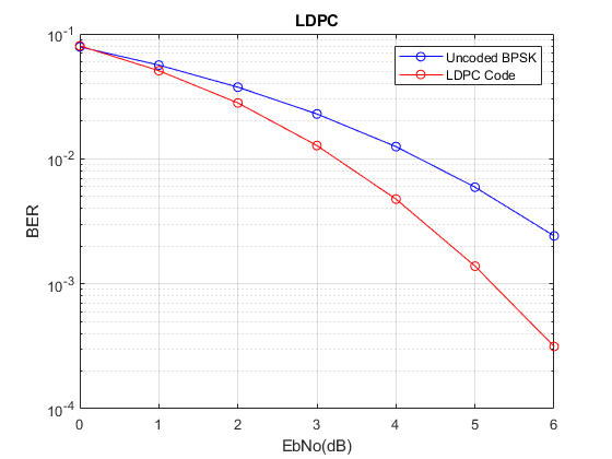
The BER results show that great performance gains can be achieved over the no coding case at low to moderate signal to noise ratios. When compared with other Block Codes it is seen that this scheme achieves the same BER performance as Hamming Code (7,4) with Maximum Likelihood Decoding. This is quite an encouraging result because this is achieved with the simplest LDPC code we could imagine. With more complex codes the improvement in BER can be significant.
Reference
[1] Tilo Strutz, “Low Density Parity Check Codes – An Introduction”, June 09, 2016
http://www1.hft-leipzig.de/strutz/Kanalcodierung/ldpc_introduction.pdf