
What is Diffraction
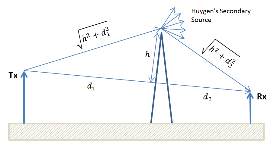
Diffraction is a phenomenon where electromagnetic waves (such as light waves) bend around corners to reach places which are otherwise not reachable i.e. not in the line of sight. In technical jargon such regions are also called shadowed regions (the term again drawn from the physics of light). This phenomenon can be explained by Huygen’s principle which states that “as a plane wave propagates in a particular direction each new point along the wavefront is a source of secondary waves”. This can be understood by looking at the following figure. However one peculiarity of this principle is that it is unable to explain why the new point source transmits only in the forward direction.

Diffraction is Difficult to Model
The electromagnetic field in the shadowed region can be calculated by combining vectorially the contributions of all of these secondary sources, which is not an easy task. Secondly, the geometry is usually much more complicated than shown in the above figure. For example consider a telecom tower transmitting electromagnetic waves from a rooftop and a pedestrian using a mobile phone at street level. The EM waves usually reach the receiver at street level after more than one diffraction (not to mention multiple reflections). However, an approximation that works well in most cases is called knife edge diffraction, which assumes a single sharp edge (an edge with a thickness much smaller than the wavelength) separates the transmitter and receiver.
Knife Edge Model
The path loss due to diffraction in the knife edge model is controlled by the Fresnel Diffraction Parameter which measures how deep the receiver is within the shadowed region. A negative value for the parameter shows that the obstruction is below the line of sight and if the value is below -1 there is hardly any loss. A value of 0 (zero) means that the transmitter, receiver and tip of the obstruction are all in line and the Electric Field Strength is reduced by half or the power is reduced to one fourth of the value without the obstruction i.e. a loss of 6dB. As the value of the Fresnel Diffraction Parameter increases on the positive side the path loss rapidly increases reaching a value of 27 dB for a parameter value of 5. Sometimes the exact calculation is not needed and only an approximate calculation, as proposed by Lee in 1985, is sufficient.
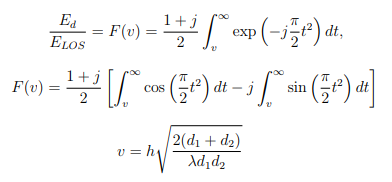
Fresnel Diffraction Parameter (v) is defined as:
v=h√(2(d1+d2)/(λ d1 d2))
where
d1 is the distance between the transmitter and the obstruction along the line of sight
d2 is the distance between the receiver and the obstruction along the line of sight
h is the height of the obstruction above the line of sight
and λ is the wavelength
The electrical length of the path difference between a diffracted ray and a LOS ray is equal to φ=(π/2)(v²) and the normalized electric field produced at the receiver, relative to the LOS path is e-jφ. Performing a summation of all the exponentials above the obstruction (from v to positive infinity) gives us the Fresnel Integral, F(v).
Plot of Diffraction Loss
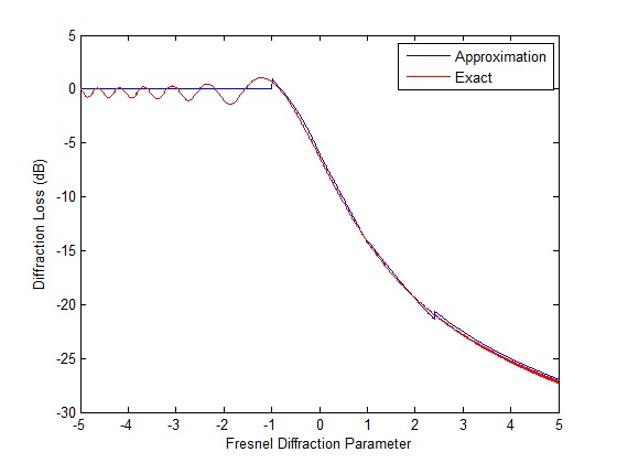
The MATLAB codes used to generate the above plots are given below (approximate method followed by the exact method). Feel free to use them in your simulations and if you have a question drop us a comment.
MATLAB Code for Approximate Calculation of Diffraction Loss
%%%%%%%%%%%%%%%%%%%%%%%%%%%%%%%%%%%%%%%%%%%%%%%%%%%%
% Calculation of the path loss based on the value of
% Fresnel Diffraction Parameter as proposed by Lee
% Lee W C Y Mobile Communications Engineering 1985
% Copyright www.raymaps.com %%%%%%%%%%%%%%%%%%%%%%%%%%%%%%%%%%%%%%%%%%%%%%%%%%%%
clear all
close all
v=-5:0.01:5;
for n=1:length(v)
   if v(n) <= -1
      G(n)=0;
   elseif v(n) <= 0
      G(n)=20*log10(0.5-0.62*v(n));
   elseif v(n) <= 1
      G(n)=20*log10(0.5*exp(-0.95*v(n)));
   elseif v(n) <= 2.4
      G(n)=20*log10(0.4-sqrt(0.1184-(0.38-0.1*v(n))^2));
   else
      G(n)=20*log10(0.225/v(n));
   end
end
plot(v, G, 'b')
xlabel('Fresnel Diffraction Parameter')
ylabel('Diffraction Loss (dB)')
MATLAB Code for Exact Calculation of Diffraction Loss
%%%%%%%%%%%%%%%%%%%%%%%%%%%%%%%%%%%%%%%%%%%%
% Exact calculation of the path loss (in dB)
% based on Fresnel Diffraction Parameter (v)
% T S Rappaport Wireless Communications P&P
% Copyright www.raymaps.com
%%%%%%%%%%%%%%%%%%%%%%%%%%%%%%%%%%%%%%%%%%%%
clear all
close all
v=-5:0.01:5;
for n=1:length(v)
   v_vector=v(n):0.01:v(n)+100;
   F(n)=((1+1i)/2)*sum(exp((-1i*pi*(v_vector).^2)/2));
end
F=abs(F)/(abs(F(1)));
plot(v, 20*log10(F),'r')
xlabel('Fresnel Diffraction Parameter')
ylabel('Diffraction Loss (dB)')
We have used the following equations in the exact calculation of the Diffraction Loss [1] above. We did not want to scare you with the math so have saved it for the end.
Also please checkout this interesting video explaining the phenomenon of diffraction.
[1] http://www.waves.utoronto.ca
21 thoughts on “Knife Edge Diffraction Model”
quotation:
[
for n=1:length(v)
v_vector=v(n):0.01:v(n)+100;
F(n)=((1+1i)/2)*sum(exp((-1i*pi*(v_vector).^2)/2));
end
]
in this section of code, why did you choose 100 as the limit of intergral? I tried to use 1000 instead of 100 but the result was not good.
I find that strange.
Question on “Knife Edge REFRACTION” a term I stumbled into researching the best over-the-air antenna for my house, 35 miles from a 400 ft high transmission tower on a 3500 ft high mountain, but halfway between there’s a 3900 ft mountain.
The article claimed the signal would drop down (to our house at 2,300′) and reach our place from “knife edge refraction”. Is this similar to your explanation? They even included a photo of a man who placed his OTA antenna near the ground on top of a rose bush. I’d send it to you but can’t on this format. It’s in front of and on the side of a hill with a pond below it.
Thank you if you answer. Kim Eastman
I guess it should work but 35 miles is a large distance. You also might want to find out what is the transmit power of the transmission tower. Plug in the numbers in FRIIS free space line of sight equation to get some idea. Hope this helps…
How do you calculate h when height of Transmitter and Receiver is different?
Also your definition of d1 and d2 does not match with the definition of ITU-R P.526-15.
Hi Raj,
If the heights are different you draw a straight line between Tx and Rx. Then draw a perpendicular from this line to tip of the obstruction. This gives you the height(h). I would suggest you look at the figure again, with the above explanation in mind.
Hope this helps!
YA
How do I minimize edge diffraction in parabolic antenna
Is that (v) ranging from -5 to 5 on the X axis? So why do we have negative (v) given that its a function of distances, height and wavelength which all are positive?
That’s an excellent question. I think it has to do with height ‘h’, which is negative when the obstruction is below the line of sight. When ‘h’ is negative, Fresnel Diffraction Parameter ‘v’ is also negative. Hope this clarifies it.
Hi John,
First of all: thanks for the nice figures and explanations.
But are you sure that h is negative when the obstruction is BELOW the line of sight and not ABOVE?
As far as I know, the oscillations occur in the shadow regime of the obstruction but according to the v-parameter and the assumption that h is negative when the obstruction is below the line of sight the oscillations occur in the lit regime.
Best regards,
Dennis Neumann
Is there another way for Fresnel Diffraction Parameter to be negative? without h being negative.
Hello Jhon,
Could you explain that why theoritical plot (red) shows higher peak than other constructive fringes in Line of sight propagation when v = -1. ( fringes are weak when v = -2, -3 …. than v = -1 )
Rafiq,
That’s a very valid question and needs investigation. However, an intuitive explanation for this (higher peak of the red curve when v=-1) is that when the obstruction is just below the line of sight the paths of the rays are not that dissimilar and the rays combine constructively. When v=-2,-3,-4 the path lengths are quite different and hence rays do not add up constructively. Makes sense?
John
Therefore, I can say that,
1. the shortest path between receiver and transmitter in LOS zone at v = -1.
2. At this position, receiver receives direct signal without any interuptions(i.e. no reflected signal) that gives us higher peak.
Am I right ?
Maybe. But we cannot say there is no interruption at all. Think of the situation when lets say v=-5 as opposed to v=-1. I think this is not as straight forward as one might think.
I agree with you.
But, another point that I noticed, interference fringes are much slower while v is increasing. I think that, it shows multiple slit(multipath effect) interference pattern when v = -5 to -3, then we get multiple slit diffraction pattern that gives us maximum intensity only at v = -1.
What do you think ?
I would suggest that you re-visit Huygens Principle of Wave Propagation. It might be helpful!
Hello John,
I have received signal from the satellite(SNR vs Time plot). Now, I would like to compare with theoretical graph regarding my practical conditions. How I can plot theoretical graph using my practical parameters. I don’t understand which formula I should use in MATLAB (above practical plot is SNR vs Position)?
Could you give some tips ?
This post is about diffraction. I do not see the relevance to your problem. There must be models for satellite signal attenuation with distance. The most simple is Free Space Model (also called Friis Model).
Hello Jhon,
Could you explain that why theoritical plot (red) shows higher peak than other constructive fringes in Line of sight propagation when v = -1. ( fringes are weak when v = -2, -3 …. than v = -1 ).
Please don’t spam, but think on your own. What does the Huygens principle tell?