A sinusoidal signal is the most fundamental type of signal that exists in communication systems, power systems, navigation systems etc. It is controlled by three parameters which are the amplitude, phase and frequency. The last two, that is phase and frequency, are interconnected. As discussed in my previous post Instantaneous Frequency (IF) is nothing but the rate of change of phase. This can be mathematically described as:
IF=Δφ/Δt
It is sometimes important in communication systems to estimate the phase and frequency of the signal arriving at the receiver. This is especially true for Phase Modulated (PM) and Frequency Modulated (FM) systems. But any synchronous communication system requires that the carrier phase and frequency is synchronized between the transmitter and receiver. For more on carrier phase and frequency synchronization error please see my previous post.
There are number of ways to estimate the frequency of a sine wave, from Fast Fourier Transform (FFT), to Autoregressive (AR) methods, to high resolution spectral estimation methods such as MUSIC* and ESPRIT**. The challenge here is to perform an accurate estimation with minimum number of samples and in presence of high noise and interference. Sometimes it is also required to detect multiple sinusoids simultaneously, which are overlapping in time domain and closely spaced in the frequency domain.
In this post we present the simplest method of frequency estimation that is called the Zero Crossing (ZC) method. Since a sine wave crosses the x-axis twice during each cycle, we can simply count the number of crossings and divide it by two and again divide it by the observation window size, giving us the frequency in Hertz. Please note that for this scheme to work we need to have a few complete cycles. Higher the length of the observation window greater is the accuracy.
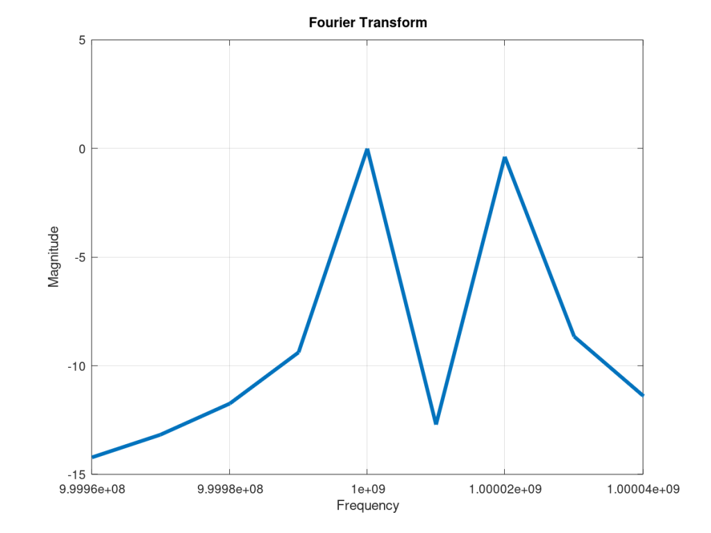
It has been shown in [1] that at high Signal to Noise Ratio (SNR > 10dB) ZC estimator approaches the Cramer Rao Lower Bound (CRLB). MATLAB code for the ZC method is given below. For comparison we have also included the FFT method in our simulation and results are shown in the figure below. Please remember that accuracy of the FFT method depends upon the window size T in the time domain. Mathematically, the frequency bin size is given as:
Δf=1/T
To separate two sinusoids the minimum separation must be 2Δf and not Δf as there needs to be a vacant bin between the two sinusoids. Also, we experimented with the frequency resolution of Zero Crossing detector and it was found out to be Δf/2 (although, unlike FFT, this method can detect only one tone at a time). It must be noted that frequency resolution of FFT does not increase by increasing the sampling frequency. In fact if sampling frequency is increased and number of samples remains the same, frequency resolution in fact decreases.
%%%%%%%%%%%%%%%%%%%%%%%%%%%%%%%%%
%     FREQUENCY ESTIMATION
%            USING
%     ZERO CROSSING METHOD
%       www.raymaps.com
%%%%%%%%%%%%%%%%%%%%%%%%%%%%%%%%%
clear all
close all

N=1e6;              % Number of samples
fc=1e9;             % Carrier frequency
fs=10*fc;           % Sampling frequency
ts=1/fs;            % Sampling interval
t=0:ts:N*ts;        % Total time
dp=pi/6;            % Phase offset
df=20e3;            % Frequency offset

tx_carrier=sqrt(2)*cos(2*pi*fc*t);
rx_carrier=sqrt(2)*cos(2*pi*(fc+df)*t+dp)+0.1*randn(1,N+1);

% Frequency Estimation at Transmitter
count=0;
for n=1:N
  if tx_carrier(n)>0 && tx_carrier(n+1)<0   % -ve going
    count=count+1;
  end
  if tx_carrier(n)<0 && tx_carrier(n+1)>0   % +ve going
    count=count+1;
  end
end
tx_freq_estimate=count/2/t(end)

% Frequency Estimation at Receiver
count=0;
for n=1:N
  if rx_carrier(n)>0 && rx_carrier(n+1)<0   % -ve going
    count=count+1;
  end
  if rx_carrier(n)<0 && rx_carrier(n+1)>0   % +ve going
    count=count+1;
  end
end
rx_freq_estimate=count/2/t(end)

% Fourier Transform
two_tones=tx_carrier+rx_carrier;
fft_two_tones=abs(fft(two_tones));
fft_two_tones=fft_two_tones/max(fft_two_tones);
f=0:1/t(end):(N)*(1/t(end));
plot(f,10*log10(fft_two_tones),'linewidth',3);
axis([fc-2*df fc+2*df -15 5])
xlabel('Frequency')
ylabel('Magnitude')
title('Fourier Transform')
grid on
Note: The frequency estimate of Zero Crossing method can be improved greatly by using a simple Moving Average (MA) filter before the detection of Zero Crossings.
Complex Exponential
Sometimes the signal is not real (sinusoid) but is complex in nature (exponential). For such a case the above code can be slightly modified to do the Zero Crossing calculation. The method we adopt is to do the Zero Crossing calculation for both the real and imaginary parts separately and then take the average. The noise that is added to the signal is also complex in nature now. Last thing we want to mention is that applying a Moving Average filter just before the ZC algorithm greatly improves the estimate. The MATLAB/Octave code for this is given below.
%%%%%%%%%%%%%%%%%%%%%%%%%%%%%%%%%
%     FREQUENCY ESTIMATION
%            USING
% ZERO CROSSING METHOD (COMPLEX)
%       www.raymaps.com
%%%%%%%%%%%%%%%%%%%%%%%%%%%%%%%%%
clear all
close all

N=1000;             % Number of samples
fc=1e9;             % Carrier frequency
fs=10*fc;           % Sampling frequency
ts=1/fs;            % Sampling interval
t=0:ts:N*ts;        % Total time
dp=2*pi*(rand-0.5); % Random phase offset
df=1e6*(rand-0.5);  % Random frequency offset

white_noise=sqrt(0.1/2)*(randn(1,N+1)+i*randn(1,N+1));
tx_carrier=exp(i*2*pi*fc*t);
rx_carrier=exp(i*2*pi*(fc+df)*t+dp)+white_noise;
rx_carrier=conv(rx_carrier, ones(1,5),'same');

% Frequency Estimation at Receiver (Real Part)
count1=0;
for n=1:N
  if real(rx_carrier(n))>0 && real(rx_carrier(n+1))<0   % -ve going
    count1=count1+1;
  end
  if real(rx_carrier(n))<0 && real(rx_carrier(n+1))>0   % +ve going
    count1=count1+1;
  end
end

% Frequency Estimation at Receiver (Imaginary Part)
count2=0;
for n=1:N
  if imag(rx_carrier(n))>0 && imag(rx_carrier(n+1))<0   % -ve going
    count2=count2+1;
  end
  if imag(rx_carrier(n))<0 && imag(rx_carrier(n+1))>0   % +ve going
    count2=count2+1;
  end
end

rx_freq_estimate=mean([count1/2/t(end) count2/2/t(end)]);
freq_error=(fc+df)-rx_freq_estimate
[1] Yizheng Liao, “Phase and Frequency Estimation: High-Accuracy and Low-Complexity Techniques,” MS Thesis Worcester Polytechnic Institute, May 2011.
* MUSIC: Multiple Signal Classification
** ESPRIT: Estimation of Signal Parameters via Rotational Invariance Technique