Tag Archives: BER

Bit Error Rate of QPSK in Rayleigh Fading

So far we have considered the bit error rate (BER) of BPSK and QPSK in an AWGN channel. Now we turn our attention to a Rayleigh fading channel which is a more realistic representation of a wireless communication channel. We consider a single tap Rayleigh fading channel which is good approximation of a flat fading channel i.e. a channel that has flat frequency response (but varying with time). The complex channel coefficient is given as (a+j*b) where a and b are Gaussian random variables with mean 0 and variance 0.5. We use the envelope of this channel coefficient in our simulation as any phase shift is easily removed by the receiver.

%%%%%%%%%%%%%%%%%%%%%%%%%%%%%%%%%%%%%%%%
function[ber]=err_rate3(l,EbNo)
si=2*(round(rand(1,l))-0.5);
sq=2*(round(rand(1,l))-0.5);
s=si+j*sq;
n=(1/sqrt(2*10^(EbNo/10)))*(randn(1,l)+j*randn(1,l));
h=(1/sqrt(2))*((randn(1,l))+j*(randn(1,l)));
r=abs(h).*s+n;
si_=sign(real(r));
sq_=sign(imag(r));
ber1=(l-sum(si==si_))/l;
ber2=(l-sum(sq==sq_))/l;
ber=mean([ber1 ber2]);
return
%%%%%%%%%%%%%%%%%%%%%%%%%%%%%%%%%%%%%%%%

It is observed that the BER for a Rayleigh fading channel is much higher than the BER for an AWGN channel. In fact, for Rayleigh fading, the BER curve is almost a straight line!!!

Rayleigh Fading

Note:

1. The input EbNo to the function is in dB so it is converted into linear scale by 10^(EbNo/10).

2. Noise is added in a Rayleigh fading channel as well. Noise is introduced by the receiver front end and is always present.

Bit Error Rate of QPSK

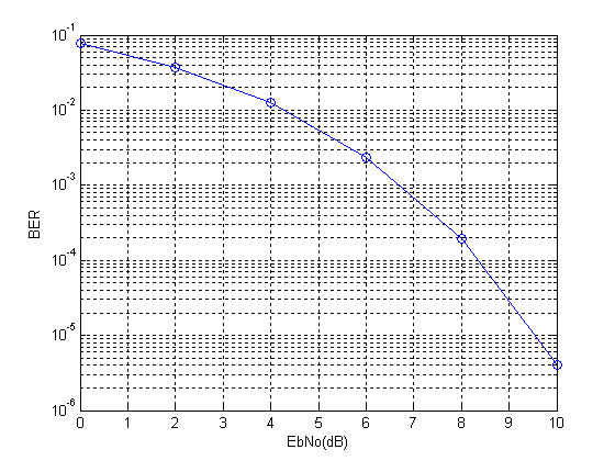
Simulating a QPSK system is equivalent to simulating two BPSK systems in parallel. So there is no difference in bit error rate(BER). Since the simulation is at baseband we multiply the in-phase and quadrature streams by 1 and j respectively (instead of cos and sin carriers). At the receiver we just use the real and imag functions to separate the two symbol streams. The BER is the average BER of the two parallel streams.

As in the case of BPSK we can show that the baseband representation (using 1 and j)  is equivalent to using the passband representation (using cosine and sine). Lets assume the following signal model for QPSK.

s(t)=a(t)*cos(2*pi*f*t)+b(t)*sin(2*pi*f*t)

where a(t) and b(t) contain the information to be transmitted over the channel. Now at the receiver we multiply this signal with cos( ) to recover a(t) and sin( ) to recover b(t).

cos(2*pi*f*t)*s(t)

=cos(2*pi*f*t) [a(t)*cos(2*pi*f*t)+b(t)*sin(2*pi*f*t)]

=a(t)*cos(2*pi*f*t)*cos(2*pi*f*t) +b(t)*sin(2*pi*f*t)*cos(2*pi*f*t)

=(a(t)/2)*(1+cos(4*pi*f*t))+(b(t)/2)*sin(4*pi*f*t)

=(a(t)/2)+(a(t)/2)*cos(4*pi*f*t)+(b(t)/2)*sin(4*pi*f*t)

After low pass filtering (LPF) we get (a(t)/2), which it the required in-phase component scaled by a constant 1/2. Similarly we can find the quadrature component b(t).

sin(2*pi*f*t)*s(t)

=sin(2*pi*f*t) [a(t)*cos(2*pi*f*t)+b(t)*sin(2*pi*f*t)]

=a(t)*sin(2*pi*f*t)*cos(2*pi*f*t)+b(t)*sin(2*pi*f*t)*sin(2*pi*f*t)

=(a(t)/2)*sin(4*pi*f*t)+(b(t)/2)*(1-cos(4*pi*f*t))

=(a(t)/2)*sin(4*pi*f*t)+(b(t)/2)-(b(t)/2)cos(4*pi*f*t)

Again after low pass filtering (LPF) we are left with the quadrature component b(t) scaled by the constant 1/2. So we can conclude that the multiplication by the carrier terms at the transmitter and receiver is not required in simulation and we can simply transmit a(t) and b(t). We just have to make sure that a(t) and b(t) are orthogonal to each other so that they do not interfere.

So the transmitted QPSK signal would have the form.

s(t)=a(t)+j*b(t)

The steps involved in the simulation are

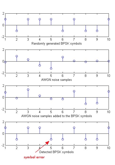
1. Generate a random sequence of symbols for the in-phase and quadrature components (-1 corresponding to binary value of 0 and +1 corresponding to binary value of 1). Add the in-phase and quadrature components in the form a(t)+j*b(t).

2. Generate complex samples of Additive White Gaussian Noise (AWGN) with the required variance (noise power = noise variance OR noise power = square of noise standard deviation OR noise power = noise power spectral density * signal bandwidth).

3. Add AWGN samples to the QPSK signal.

4. Detection is performed at the receiver by determining the sign of the in-phase and quadrature components.

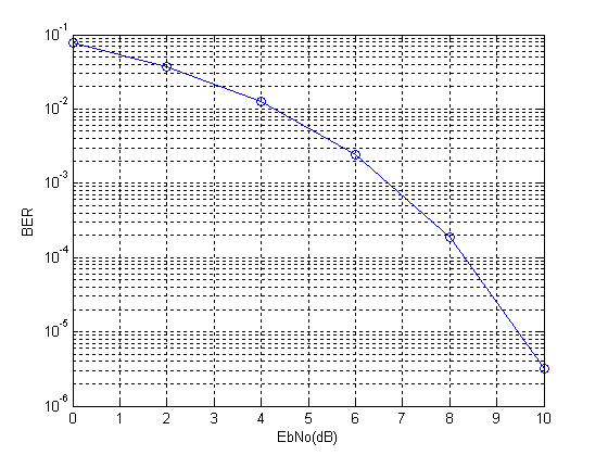
5. And finally the bit error rate (BER) is calculated for the in-phase and quadrature components. Total bit error rate is the mean of the two values.

%%%%%%%%%%%%%%%%%%%%%%%%%%%%%%%%%%%%%%%%%%%%%%%%%%%%%%%%%%%%%%%%%%%%%%%%%%%%
% FUNCTION TO CALCULATE BER OF QPSK IN AWGN
% l - Input, length of the symbol sequence
% EbNo - Input, energy per bit to noise power spectral density
% ber - Output, bit error rate
%%%%%%%%%%%%%%%%%%%%%%%%%%%%%%%%%%%%%%%%%%%%%%%%%%%%%%%%%%%%%%%%%%%%%%%%%%%%
function[ber]=err_rate2(l,EbNo)       
si=2*(round(rand(1,l))-0.5);               % In-phase component
sq=2*(round(rand(1,l))-0.5);               % Quadrature component
s=si+j*sq;                              % QPSK symbol  
n=(1/sqrt(2*10^(EbNo/10)))*(randn(1,l)+j*randn(1,l)); % AWGN Noise
r=s+n;                                  % Received signal with noise
si_=sign(real(r));                        % Detected in-phase component 
sq_=sign(imag(r));                        % Detected quadrature component 
ber1=(l-sum(si==si_))/l;                  % Bit error rate in-phase
ber2=(l-sum(sq==sq_))/l;                  % Bit error rate quadrature
ber=mean([ber1 ber2]);                    % Mean bit error rate 
return
%%%%%%%%%%%%%%%%%%%%%%%%%%%%%%%%%%%%%%%%%%%%%%%%%%%%%%%%%%%%%%%%%%%%%%%%%%%%

QPSK Constellation

QPSK BER

One final comment that I want to make is that bit error rate and symbol error rate is not always the same. Taking the example of QPSK a symbol error might occur when there is an error in the in-phase stream or the quadrature stream or both. So it is not a one to one mapping!!!

Note:

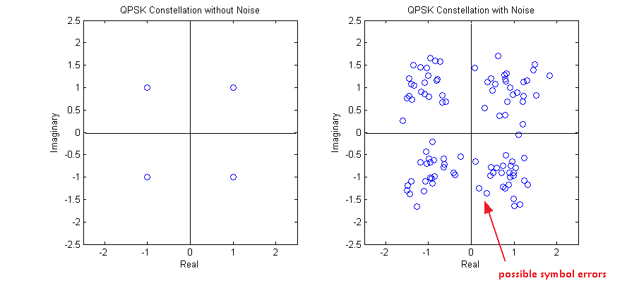
1. For a QPSK constellation centered around the origin of the co-ordinate system, the decision boundaries are simply defined by the x and y axes.

2. The reason for the name QPSK is that there are four symbols in the constellation, each having one of four possible phases (45, 135, 225, 315).

Bit Error Rate of BPSK

Modulation is the process by which a binary stream (zeros and ones) is converted to a format that is suitable for transmission over a wired or wireless channel that is prone to noise and interference as well as distortion. The most basic modulation scheme is BPSK or Binary Phase Shift Keying. It transmits the information in the phase of the signal which could be one of two values (0 degrees or 180 degrees).

BPSK signal can be represented as (called the passband representation)

s(t)=a(t)*cos(2*pi*f*t)

where a(t) is a time varying parameter which can have one of two values (+1 or -1). This is equivalent to having the phase of the carrier rotated by 0 degrees or 180 degrees. In simulation of digital communications systems we usually take out the carrier and perform the simulation at baseband. The passband and baseband simulations are equivalent because the carrier signal introduced at the transmitter can be easily removed at the receiver by a process called correlation (or simply put multiplication by the carrier followed by low pass filtering) and what we are left with is the parameter a(t).

If the transmitted signal is given as

a(t)*cos(2*pi*f*t)

then by multiplication with the carrier at the receiver we get

a(t)*cos(2*pi*f*t)*cos(2*pi*f*t)

=(a(t)/2)*(1+cos(4*pi*f*t))

and after low pass filtering the cosine term at twice the carrier frequency is removed and we get the parameter a(t) scaled by the factor 1/2. Since the information is contained in the sign of the parameter a(t) we can recover our transmitted symbols.

So in simulation, instead of multiplying the parameter a(t) by the carrier at transmitter and then again at the receiver we simply transmit a(t). This is equivalent to simulation of a Pulse Amplitude Modulation (PAM) system with two levels. Following are the steps involved in the simulation of BPSK system.

Steps:

1. Generate a random sequence of symbols (+1,-1)

2. Generate samples of Additive White Gaussian Noise (AWGN) with the required variance (noise power = noise variance OR noise power = square of noise standard deviation OR noise power = noise power spectral density * signal bandwidth).

3. Add AWGN samples to the BPSK signal.

4. Detection is performed at the receiver by determining the sign of the parameter a(t).

5. And finally the bit error rate (BER) is calculated. Which is the same as symbol error rate (SER) in this case.

Given below is the MATLAB code that performs these functions. Also shown below are the signals generated at the first four steps and the bit error rate calculated in the fifth and last step.

%%%%%%%%%%%%%%%%%%%%%%%%%%%%%%%%%%%%%%%%%%%%%%%%%%%%%%%%%%%%%%%%%%%%%
% FUNCTION TO CALCULATE BER OF BPSK IN AWGN
% l - Input, length of the symbol sequence
% EbNo - Input, energy per bit to noise power spectral density in dB
% ber - Output, bit error rate
%%%%%%%%%%%%%%%%%%%%%%%%%%%%%%%%%%%%%%%%%%%%%%%%%%%%%%%%%%%%%%%%%%%%%
function[ber]=err_rate(l,EbNo)
s=2*(round(rand(1,l))-0.5);             % Generate BPSK symbols 
n=(1/sqrt(2*10^(EbNo/10)))*randn(1,l);  % Generate AWGN noise
r=s+n;                                  % Add noise to signal
s_=sign(r);                             % Detect symbols
ber=(l-sum(s==s_))/l;                   % Calculate BER
return
%%%%%%%%%%%%%%%%%%%%%%%%%%%%%%%%%%%%%%%%%%%%%%%%%%%%%%%%%%%%%%%%%%%%%

The length of the symbol sequence and EbNo (a bit different than SNR) are the inputs to the function and the bit error rate (BER) is the output. The length of the sequence must be such that you can count about 25 symbol errors at each value of EbNo. This means that at an EbNo of 10dB you would need to pass a few million symbols through the channel. Try it out!!!

BPSK Modulation

BPSK BER

Note:

1. To generate the above given bit error rate plot you would have to create a piece of code which calls the above function for each value of EbNo and stores the output BER value in an array and then plot the BER vs EbNo at the end of simulation. We leave this to  you as an exercise.

2. We have generated BPSK symbols directly instead of first generating a binary sequence. This does not matter much in this simple example but for more advanced modulation schemes we would have to first generate a binary stream and then from that the symbols.

3. We have used one sample per symbol of BPSK modulation, as shown in the figure above. But sometimes we have to select higher number of samples per symbol (usually 4 to 10) to implement some other signal processing functions.

4. Most of the concepts discussed above can be extended to other digital modulation schemes. The concepts for analog modulation schemes are somewhat different and we do not use error rates to evaluate the performance of these schemes.