
Some Background
In a previous post we calculated the Bit Error Rate (BER) of a Massive MIMO system using two different channel models namely deterministic and probabilistic. The deterministic channel model is derived from the geometry of the array (ULA in this case) and the distribution of users in the cell. Whereas probabilistic channel model assumes that the channel is flat fading and can be modeled, between each transmit receive pair, as a complex, circularly symmetric, Gaussian random variable with mean of zero and variance of 0.5 per dimension.
We observed that the BER performance of a Massive MIMO system was orders of magnitude better in a probabilistic channel than in a deterministic channel. We also discussed why this is the case and how we can make a fair comparison between the two. One suggestion we gave was to adjust the Signal to Noise Ratio (SNR) in the complex Gaussian channel as the assumption of multipath-rich scattering environment which yields IID (Independent and Identically Distributed) channel coefficients also dictates that the SNR must be much lower due to reflection, refraction, diffraction and scattering (see figure below for an example of multipath-rich scattering environment).
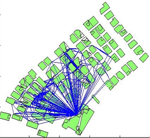
from Ray Tracing Simulator by Usman Sheikh
Antenna Correlation Models
One point that we did not discuss, at least not in detail, was that the IID assumption is not valid in a realistic channel where there is always some correlation between the antenna elements. Smaller the separation between antenna elements greater is the correlation. Correlation is also greater at the Base Station (BS) than at the Mobile Station (MS) as the angles of arrival at the BS are much narrower. The question is how we can model this correlation as a function of antenna spacing. There are three options that we have, namely (i) Uniform Correlation (ii) Exponential Correlation (iii) Bessel Correlation [1]. We chose the Exponential Model as it is intuitive and quite easy to implement. According to this model correlation between antenna m and antenna n of an array if given as:
ρm,n=exp(-xm,n/xo)
Where xm,n is the separation between the antenna elements m and n and xo is a constant which controls the level of correlation. For a Mobile Station the value of this constant would be around half a wavelength whereas for a base station it could be as high as tens of wavelengths. Higher the value of xo greater is the correlation between the pair of antenna elements under consideration. The channel matrix Hc with the appropriate channel correlation can then be written as [2]:
Hc=(RBS1/2)(H)(RMS1/2)
Where RBS and RMS are matrices of correlation coefficients at the Base Station (receiver) and Mobile Station (transmitter) respectively. The diagonal elements of the correlation matrices are one and non-diagonal elements decrease exponentially as you move further away (for immediate neighbors the correlation is defined as 0.3, 0.7 and 0.9 for low, medium and high correlation respectively). For no spatial correlation case the correlation matrices simplify to identity matrices i.e. the non-diagonal terms are all zero.
Simulation Results
CASE 1: No correlation
CASE 2: MS low (0.3), BS low (0.3)
CASE 3: MS low (0.3), BS medium (0.7)
CASE 4: MS low (0.3), BS high (0.9)
In the brackets above we give the level of correlation with the nearest neighbor. This decreases exponentially as we move to elements further from the element of interest. We observe that antenna correlation does have great impact on the BER performance of a Massive MIMO system and the difference that we previously saw between the deterministic channel and the probabilistic channel results is somewhat diminished.
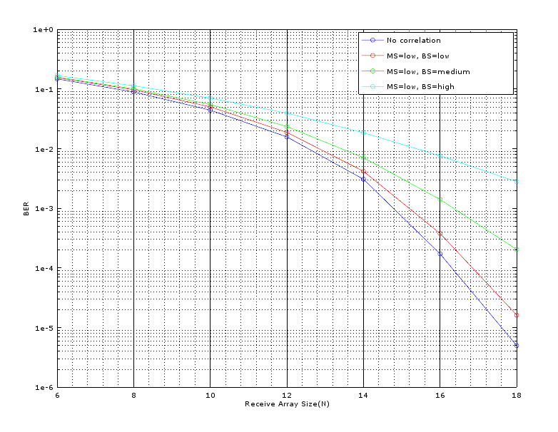
(M=16, N=6,8,10,12,14,16,18)
MATLAB Code
Main Function Containing the Linear Processors
%%%%%%%%%%%%%%%%%%%%%%%%%%%%%%%%%%%%
% MASSIVE MIMO PROCESSING
% IN CORRELATED ENVIRONMENT
% COPYRIGHT RAYMAPS (C) 2019
%%%%%%%%%%%%%%%%%%%%%%%%%%%%%%%%%%%%
function [ber]=Massive_MIMO(M,N,R_MS,R_BS,EbNo)

% SETTING THE PARAMETERS FOR THE SIMULATION
f=1e9;                     %Carrier frequency
c=3e8;                     %Speed of light
l=c/f;                     %Wavelength
%d=l/2;                    %Rx array spacing
%theta=2*pi*(rand(1,M));   %Angular separation of users
sigma=1/sqrt(2*EbNo);      %Standard deviation of noise

n=1:N;                     %Rx array number
n=transpose(n);            %Row vector to column vector

% RECEIVE SIGNAL MODEL (LINEAR)
s=2*(round(rand(M,1))-0.5);           %BPSK signal of length M
%H=exp(-i*(n-1)*2*pi*d*cos(theta)/l); %Deterministic channel NxM
H=(1/sqrt(2))*(randn(N,M)+i*randn(N,M));%Probabilistic channel NxM
H=sqrtm(R_BS)*H*sqrtm(R_MS);          %Introducing correlation in H
wn=sigma*(randn(N,1)+i*randn(N,1));   %AWGN noise of length N
x=H*s+wn;                             %Receive vector of length N

% LINEAR ARRAY PROCESSING - METHODS
% 1-MATCHED FILTER
% y=H'*x;

% 2-PINV without tol
% y=pinv(H)*x;

% 3-PINV with tol
% y=pinv(H,0.1)*x;

% 4-Minimum Mean Square Error (MMMSE)
y=(H'*H+(2*sigma^2)*eye([M,M]))^(-1)*(H')*x;

% DEMODULATION AND BER CALCULATION
s_est=sign(real(y));          %Demodulation
ber=sum(s!=s_est)/length(s);  %BER calculation

% Please remove % in front of the array processing technique
% you want to implement (1-MF, 2-LS1, 3-LS2, 4-MMSE)

return
Wrapper for Generating the BER Graphs
clear all               %Clear all variables
%close all              %Close all figures

EbNodB=10;              %EbNo on dB scale
EbNo=10^(EbNodB/10);    %EbNo on linear scale
N_vector=2:2:18;        %Rx array length range
M=16;                   %Tx array length (or users)

for j=1:length(N_vector)%Varying the length of the receive array
  N=N_vector(j);        %Selecting a value of N

  R_MS=eye(M,M);        %Initializing R_MS
  R_BS=eye(N,N);        %Initializing R_BS

  for p=1:M
    for q=1:M
      R_MS(p,q)=exp(-abs(p-q));   %Correlation coefficient
    end
  end

  for p=1:N
    for q=1:N
      R_BS(p,q)=exp(-abs(p-q)/10);%Correlation coefficient
    end
  end

  for k=1:50000               %This number may be increased
    [ber]=Massive_MIMO(M,N,R_MS,R_BS,EbNo); %Main function
    BER_array(k)=ber;         %Storing the BER in the array
  end

BER_total(j)=mean(BER_array); %Calculating the mean BER for each N
end

semilogy(N_vector, BER_total,'ko-') %Plot on log scale
xlabel('Receive Array Size(N)')     %X-label
ylabel('BER')                       %Y-label
hold on                             %Hold on
grid on                             %Grid on
Some Concluding Thoughts
Massive MIMO is a term which is not clearly defined, some say this means tens of antennas at the transmitter and receiver others say hundreds. In the above analysis we have considered 16 transmit antennas and up to 18 receive antennas, which is a very nominal Massive MIMO scenario. To further assess the performance of the linear estimation techniques in a flat fading channel, with correlated fading, we considered 16×16, 32×32 and 64×64 scenarios. There is nothing in the simulation setup that limits you from going even further up, other than the computational power of your machine.
So as a first estimate you would think that the performance of 16×16, 32×32 and 64×64 scenarios must be similar (why?), as suggested by capacity theorems of MIMO systems. But this is not the case. The BER performance actually improves as you move to higher array configurations. At first, we thought that this has to do with the Exponential Correlation Model we have used, since the model assumes that the correlation falls rapidly as you move from nearest neighbours to more distant ones. But this is not the case the BER for higher configurations is much lower even with no correlation. This is a surprising result and we would like to investigate it further. Conclusion: This has to do with calibration of the simulation. If the transmit power is scaled to accommodate for higher number of transmit antennas the BER performance does not change as we go from M=2 to 4 or 8 or 16.
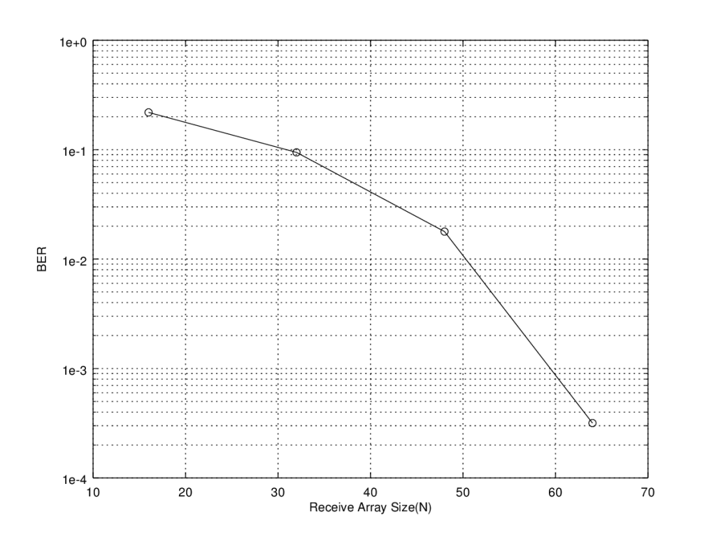
(M=64, N=16,32,48,64)
So for Massive MIMO systems it is suggested to appropriately select the level of correlation as you move to higher number of Tx-Rx combinations. From a practical point of view it is obvious that as you move to higher configurations, antennas would have to be placed much closer together thereby increasing the spatial correlation. In future we may devote a post to how the spatial correlation between antenna elements is calculated and compare the different models available.
References
[1] Xiaoming Chen, “Antenna Correlation and Its Impact on Multi-Antenna System”, Progress in Electromagnetics Research B, Vol. 62, 241–253, 2015.
[2] Ali Jemmali, Jean Conan “Investigation of the Correlation Effect on the Performance of V-BLAST and OSTBC MIMO Systems”, ICWMC 2011: The Seventh International Conference on Wireless and Mobile Communications, 2011.
Note:
- All simulations assume Binary Phase Shift Keying (BPSK) modulation unless otherwise stated. However, the simulations can easily incorporate higher order modulations such as Quadrature Amplitude Modulation (QAM).
- All simulations were carried out using MMSE processor but the code is in place to evaluate other linear estimation techniques such as MF, ZF and LS.
- As shown in the code above the number of transmit antennas M is fixed and the number of receive antennas N is varied until a sufficiently low Bit Error Rate (BER) is achieved (M=16 in first plot and M=64 in the second plot).
3 thoughts on “Massive MIMO and Antenna Correlation”
Hi sir
Would you please give the Derivation of Massive MIMO SNR under Rayleigh fading channel for BPSK
Thanking you.
Would have to dig some literature to find this.
Lets start with the basics and understand how diversity works in a simple SIMO system. We can then move to MIMO or Massive MIMO.
https://www.youtube.com/watch?v=X8CLTmlr2VM