We have previously looked at frequency domain fading simulators i.e. simulators that define the Doppler components in the frequency domain and then perform an IDFT to get the time domain signal. These simulators include Smith’s Simulator, Young’s Simulator and our very own Computationally Efficient Rayleigh Fading Simulator. Another technique that has been widely reported in the literature is Sum of Sinusoids Method. As the name suggests this method generates the Doppler components in the time domain and then sums them up to generate the time domain fading envelope. There are three parameters that define the properties of the generated signal.
1) Number of sinusoids – Higher the number better the properties of the generated signal but greater the computational complexity
2) Angle of arrival – This can be generated statistically or deterministically, spread from –pi to pi.
3) Phase of the arriving wave – This is uniformly distributed between –pi and pi.
The MATLAB code below gives three similar sum of sinusoids techniques for generating a Rayleigh faded envelope [1].
%%%%%%%%%%%%%%%%%%%%%%%%%%%%%%%%%%%%%%%%%%%%%
% SUM OF SINUSOIDS FADING SIMULATORS
% fd - Doppler frequency
% fs - Sampling frequency
% ts - Sampling period
% N - Number of sinusoids
%
% www.raymaps.com
%%%%%%%%%%%%%%%%%%%%%%%%%%%%%%%%%%%%%%%%%%%%%

clear all
close all

fd=70;
fs=1000000;
ts=1/fs;
t=0:ts:1;
N=100;

%%%%%%%%%%%%%%%%%%%%%%%%%%%%%%%%%%%%%%%%%%%%%
% Method 1 - Clarke
%%%%%%%%%%%%%%%%%%%%%%%%%%%%%%%%%%%%%%%%%%%%%
x=zeros(1,length(t));
y=zeros(1,length(t));

for n=1:N;n
    alpha=(rand-0.5)*2*pi;
    phi=(rand-0.5)*2*pi;
    x=x+randn*cos(2*pi*fd*t*cos(alpha)+phi);
    y=y+randn*sin(2*pi*fd*t*cos(alpha)+phi);
end
z=(1/sqrt(N))*(x+1i*y);
r1=abs(z);

plot(t,10*log10(r1))
hold on

%%%%%%%%%%%%%%%%%%%%%%%%%%%%%%%%%%%%%%%%%%%%%
% Method 2 - Pop, Beaulieu
%%%%%%%%%%%%%%%%%%%%%%%%%%%%%%%%%%%%%%%%%%%%%
x=zeros(1,length(t));
y=zeros(1,length(t));

for n=1:N;n
    alpha=2*pi*n/N;
    phi=(rand-0.5)*2*pi;
    x=x+randn*cos(2*pi*fd*t*cos(alpha)+phi);
    y=y+randn*sin(2*pi*fd*t*cos(alpha)+phi);
end
z=(1/sqrt(N))*(x+1i*y);
r2=abs(z);

plot(t,10*log10(r2),'r')
hold on

%%%%%%%%%%%%%%%%%%%%%%%%%%%%%%%%%%%%%%%%%%%%%
% Method 3 - Chengshan Xiao
%%%%%%%%%%%%%%%%%%%%%%%%%%%%%%%%%%%%%%%%%%%%%
x=zeros(1,length(t));
y=zeros(1,length(t));

for n=1:N;n
    phi=(rand-0.5)*2*pi;
    theta=(rand-0.5)*2*pi;
    alpha=(2*pi*n+theta)/N;
    x=x+randn*cos(2*pi*fd*t*cos(alpha)+phi);
    y=y+randn*sin(2*pi*fd*t*cos(alpha)+phi);
end
z=(1/sqrt(N))*(x+1i*y);
r3=abs(z);

plot(t,10*log10(r3),'g')
hold off

xlabel('Time(sec)')
ylabel('Envelope(dB)')
%%%%%%%%%%%%%%%%%%%%%%%%%%%%%%%%%%%%%%%%%%%%%
All the three techniques given above are quite accurate in generating a Rayleigh faded envelope with the desired statistical properties. The accuracy of these techniques increases as the number of sinusoids goes to infinity (we have tested these techniques with up to 1000 sinusoids but realistically speaking even 100 sinusoids are enough). If we want to compare the three techniques in terms of the Level Crossing Rate (LCR) and Average Fade Duration (AFD) we can say that the first and third technique are a bit more accurate than the second technique. Therefore we can conclude that a statistically distributed angle of arrival is a better choice than a deterministically distributed angle of arrival. Also, if we look at the autocorrelation of the in-phase and quadrature components we see that for the first and third case we get a zero order Bessel function of the first kind whereas for the second case we get a somewhat different sequence which approximates the Bessel function with increasing accuracy as the number of sinusoids is increased.
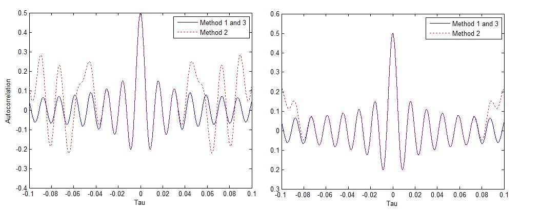
The above figures show the theoretical Bessel function versus the autocorrelation of the real/imaginary part generated by method number two. The figure on the left considers 20 sinusoids whereas the figure on the right considers 40 sinusoids. As can be seen the accuracy of the autocorrelation sequence increases considerably by doubling the number of sinusoids. We can assume that for number of sinusoids exceeding 100 i.e. N=100 in the above code the generated autocorrelation sequence would be quite accurate.
[1] Chengshan Xiao, “Novel Sum-of-Sinusoids Simulation Models for Rayleigh and Rician Fading Channels,” IEEE TRANSACTIONS ON WIRELESS COMMUNICATIONS, VOL. 5, NO. 12, DECEMBER 2006.
Author: Yasir
More than 20 years of experience in various organizations in Pakistan, the USA, and Europe. Worked with the Mobile and Portable Radio Group (MPRG) of Virginia Tech and Qualcomm USA and was one of the first researchers to propose Space Time Block Codes for eight transmit antennas. Have publsihed a book “Recipes for Communication and Signal Processing” through Springer Nature.
5 thoughts on “Sum of Sinusoids Fading Simulator”
How did you generate the autocorrelation of in-phase and quadrature components of the channel coefficients? Can you please post the matlab code for that as well?
just use MATLAB function for autocorrelation…
This is completely wrong!
There is no randn (= standard normal distributed random variable generation) in any of the 3 methods!
Yes there is, don´t you see it in the loop?
x=x+randn*cos(2*pi*fd*t*cos(alpha)+phi);
y=y+randn*sin(2*pi*fd*t*cos(alpha)+phi);
Can you please post or show me how to simulate a Rician fading channel depending on the K factor using these methods?
Thank you very much in advance.
Iskander, C. D., & Multisystems, H. T. (2008). A MATLAB-based object-oriented approach to multipath fading channel simulation. Hi-Tek Multisystems, 21.