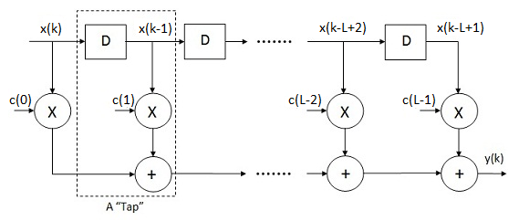
As discussed previously an LTE channel can be modeled as an FIR filter. The filter taps are described by the EPA, EVA and ETU channel models.
If x(k) is the original signal then the signal at the output of the FIR filter y(k) is given as:
y(k)=x(k)*c(0)+x(k-1)*c(1)+…..+x(k-L+2)*c(L-2)+x(k-L+1)*c(L-1)
Since the wireless channel is time varying the channel taps c(0) c(1)…..c(L-1) are also time varying with either Rayleigh or Rician distribution. It is quite easy to generate Rayleigh random variables with the desired power and distribution, however, when these Rayleigh random variables are required to have temporal correlation the process becomes a bit complicated. Temporal correlation of these variables depends upon the Doppler frequency which is turn depends upon the speed of the mobile device. The Doppler frequency is defined as:
fd=v*cos(theta)/lambda
where
fd is the Doppler Frequency in Hz
v is the receiver velocity in m/sec
lambda is the wavelength in m
and theta is the angle between the direction of arrival of the signal and the direction of motion
A simple method for generating Rayleigh random variables with the desired temporal correlation was devised by Smith [1]. His method was based on Clark and Gans fading model and has been widely used in simulation of wireless communication systems.
The method for generating the Rayleigh fading envelope with the desired temporal correlation is given below (modified from Theodore S. Rappaport Text).
1. Define N the number of Gaussian RVs to be generated, fm the Doppler frequency in Hz, fs the sampling frequency in Hz, df the frequency spacing which is calculated as df=(2*fm)/(N-1) and M total number of samples in frequency domain which is calculated as M=(fs/df).
2. Generate two sequences of N/2 complex Gaussian random variables. These correspond to the frequency bins up to fm. Take the complex conjugate of these sequences to generate the N/2 complex Gaussian random variables for the negative frequency bins up to -fm.
3. Multiply the above complex Gaussian sequences g1 and g2 with square root of the Doppler Spectrum S generated from -fm to fm. Calculate the spectrum at -fm and +fm by using linear extrapolation.
4. Extend the above generated spectra from -fs/2 to +fs/2 by stuffing zeros from -fs/2 to -fm and fm to fs/2. Take the IFFT of the resulting spectra X and Y resulting in time domain signals x and y.
5. Add the absolute values of the resulting signals x and y in quadrature. Take the absolute value of this complex signal. This is the desired Rayleigh distributed envelope with the required temporal correlation.
The Matlab code for generating Rayleigh random sequence with a Doppler frequency of fm Hz is given below.
%%%%%%%%%%%%%%%%%%%%%%%%%%%%%%%%%%%%%%%%%%%%%%%%%%%%%%%%%%%%%%%%
% RAYLEIGH FADING SIMULATOR BASED UPON SMITH'S METHOD
% N is the number of paths
% M is the total number of points in the frequency domain
% fm is the Doppler frequency in Hz
% fs is the sampling frequency in Hz
% df is the step size in the frequency domain
% Copyright RAYmaps (www.raymaps.com)
%%%%%%%%%%%%%%%%%%%%%%%%%%%%%%%%%%%%%%%%%%%%%%%%%%%%%%%%%%%%%%%%
clear all;
close all;

N=1000;
fm=300;
df=(2*fm)/(N-1);
fs=7.68e6;
M=round(fs/df);
T=1/df;
Ts=1/fs;

% Generate two sequences of N complex Gaussian random variables
g=randn(1,N/2)+j*randn(1,N/2);
gc=conj(g);
g1=[fliplr(gc), g];

g=randn(1,N/2)+j*randn(1,N/2);
gc=conj(g);
g2=[fliplr(gc), g];

% Generate Doppler Spectrum S
f=-fm:df:fm;
S=1.5./(pi*fm*sqrt(1-(f/fm).^2));
S(1)=2*S(2)-S(3);
S(end)=2*S(end-1)-S(end-2);

% Multiply the sequences with the Doppler Spectrum S, take IFFT
X=g1.*sqrt(S);
X=[zeros(1,round((M-N)/2)), X, zeros(1,round((M-N)/2))];
x=abs(ifft(X,M));

Y=g2.*sqrt(S);
Y=[zeros(1,round((M-N)/2)), Y, zeros(1,round((M-N)/2))];
y=abs(ifft(Y,M));

% Find the resulting Rayleigh faded envelope
z=x+j*y;
r=abs(z);
r=r/sqrt(mean(r.^2));

t=0:Ts:T-Ts;
plot(t,10*log10(r),'r')
xlabel('Time(sec)')
ylabel('Envelope (dB)')
axis([0 0.01 -10 5])
%%%%%%%%%%%%%%%%%%%%%%%%%%%%%%%%%%%%%%%%%%%%%%%%%%%%%%%%%%%%%%%%
The above code generates a Rayleigh random sequence with samples spaced at 0.1302 usec. This corresponds to a sampling frequency of 7.68 MHz which is the standard sampling frequency for a bandwidth of 5MHz. Similarly, the sampling rate for 10 MHz and 20 MHz is 15.36 MHz and 30.72 MHz respectively. The Doppler frequency can also be changed according to the scenario. LTE standard defines 3 channel models EPA, EVA and ETU with Doppler frequencies of 5 Hz, 70 Hz and 300 Hz respectively. These are also known as Low Doppler, Medium Doppler and High Doppler respectively.
The above code generated Rayleigh sequences of varying lengths for the three cases. But in all the cases it is in excess of 10 msec and can be used as the fading sequence for an LTE frame. Just to recall an LTE frame is of 10 msec duration with 20 time slots of 0.5 msec each. If each slot contains 7 OFDM symbols the total length of a fading sequence is 140 symbols.
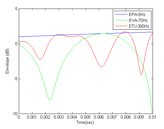
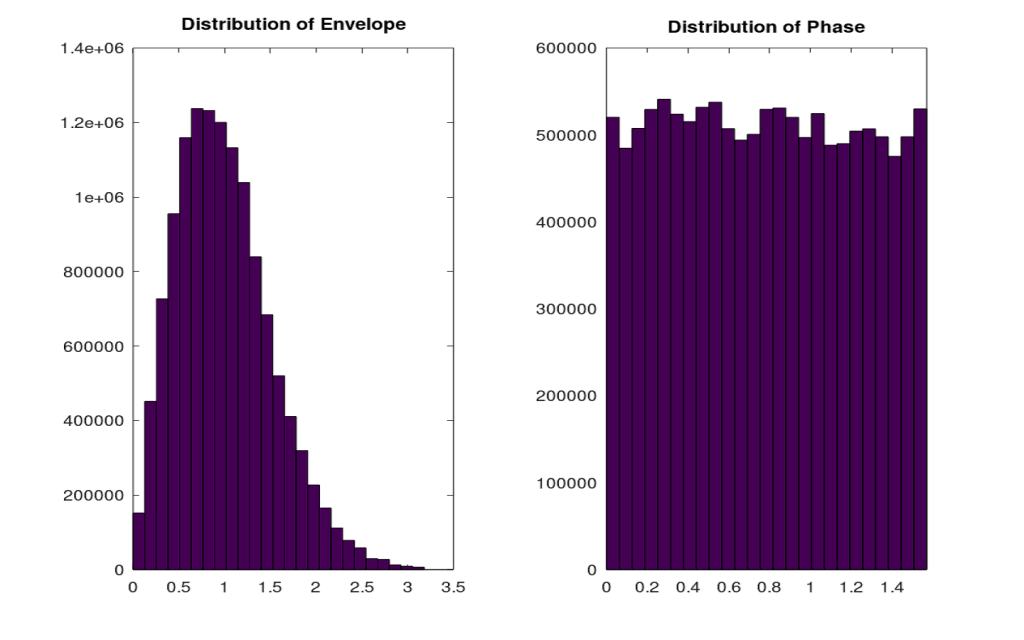
It is seen that the fluctuation in the channel increases with Doppler frequency. The channel is almost static for a Doppler frequency of 5 Hz and varies quite rapidly for a Doppler frequency of 300 Hz. It is also shown above that the envelope of z is Rayleigh distributed and phase of z is Uniformly distributed. However, the range of phase is from 0 to pi/2. This needs to be further investigated. The level crossing rate and average fade duration can also be measured.
This is the process for generating one Rayleigh distributed channel tap. This step would have to be repeated for the number of taps in the channel model which could be 7 or 9 for the LTE channel models. A Ricean distributed channel tap can be generated in a similar fashion. MIMO channel taps can also be generated using the above described method, however, we would need to understand the concept of antenna correlation before we do that.
Level Crossing Rate and Average Fade Duration
Level crossing rate (LCR) is defined as number of times per second the signal envelope crosses a given threshold. This could be either in the positive direction or negative direction. Average fade duration (AFD) is the average duration that the signal envelope remains below a given threshold once it crosses that threshold. Simply it is the average duration of a fading event. The LCR and AFD are interconnected and the product of these two quantities is a constant. The program given below calculates the LCR and AFD of the above generated envelope r.
The program calculates both the simulated and theoretical values of LCR and AFD e.g. for a threshold level of 0.3 (-5.22 dB) the LCR and AFD values calculated for fm=70 Hz and N=32 are:
LCR simulation = 45.16
LCR theoretical = 43.41
AFD simulation = 0.0015 sec
AFD theoretical = 0.0016 sec
It can be seen that the theoretical and simulation results match quite well. This gives us confidence that are generated envelope has the desired statistical characteristics.
%%%%%%%%%%%%%%%%%%%%%%%%%%%%%%%%%%%%%%%%%%%%%%%%%%%%%%
% PROGRAM TO CALCULATE THE LCR and AFD
% Rth: Level to calculate the LCR and AFD
% Rrms: RMS level of the signal r
% rho: Ratio of defined threshold and RMS level
% Copyright RAYmaps (www.raymaps.com)
%%%%%%%%%%%%%%%%%%%%%%%%%%%%%%%%%%%%%%%%%%%%%%%%%%%%%%
Rth=0.30;
Rrms=sqrt(mean(r.^2));
rho=Rth/Rrms;

count1=0;
count2=0;

for n=1:length(r)-1
     if r(n) < Rth && r(n+1) > Rth
        count1=count1+1;
     end
    if r(n) < Rth
        count2=count2+1;
    end
end
LCR=count1/(T)
AFD=((count2*Ts)/T)/LCR

LCR_num=sqrt(2*pi)*fm*rho*exp(-(rho^2))
AFD_num=(exp(rho^2)-1)/(rho*fm*sqrt(2*pi))
%%%%%%%%%%%%%%%%%%%%%%%%%%%%%%%%%%%%%%%%%%%%%%%%%%%%%%
Note:
1. According to Wireless Communications Principles and Practice by Ted Rappaport "Perform an IFFT on the resulting frequency domain signals from the in-phase and quadrature arms to get two N-length time series, and add the squares of each signal point in time to create an N-point time series. Note that each quadrature arm should be a real signal after IFFT". Now this point about the signal being real after IFFT is not always satisfied by the above program. The condition can be satisfied by playing around with the value of N a bit.
2. Also, we take the absolute value of both the time series after IFFT operation to make sure that we get a real valued sequence. However, taking the absolute value of both the in-phase and quadrature terms makes z fall in the first quadrant and the phase of z to vary from 0 to pi/2. A better approach might be to use the 'real' function instead of 'abs' function so that the phase can vary from 0 to 2pi.
3. A computationally efficient method of generating Rayleigh fading sequence is given here.
[1] John I. Smith, "A Computer Generated Multipath Fading Simulation for Mobile Radio", IEEE Transactions on Vehicular Technology, vol VT-24, No. 3, August 1975.
34 thoughts on “LTE Fading Simulator”
how to generate channel lte type Rayleigh in matlab with PDP ??
For small scale channel modeling, the power delay profile of the channel is found by taking the spatial average of the channel’s baseband impulse response over a local area. So loosely speaking channel impulse response can be derived from PDP by taking the square root of PDP. Once you have the channel impulse response you can generate the Rayleigh fading channel for each delay and perform convolution operation, after adjusting the sampling rates. This is sometimes referred to as the Tapped Delay Line Model.
Hi,
Many thanks for your post, it’s really useful.
as we know, MATLAB has some function to simulate Channel Model according 3GPP TS104: named lteFadingChannel();
But now, I can’t understand the meaning of input parameter of the function such as:
NTERM and SEED.
whether or not these values effective throughput of system. And what is correct value should we use for each specific channel model (EVA/EPA/ETU)
Could you please answer my question?
Thanks you!
I guess you would have to go through the MATLAB literature. I for one prefer using Octave instead of MATLAB and build my own functions instead of using libraries. That way you know exactly whats happening within the code!
Hi,
Thank you for sharing the codes.
it seems there is a little mistake in the code of Level crossing and AFD calculations.
In the for loop it is written
if r(n)Rth
count1=count1+1;
end
However I assume there is a mistake in if condition.
Can you point to the exact mistake that you have discovered?
Is it possible to obtain the code to generate the EPA 5Hz , EVA 70Hz profile as displayed here
Yes you can generate those by adjusting the input parameters. Do let me know if you are still struggling with it.
Is it possible to get the code for the EPA 5Hz, EVA 70Hz as displayed here in the blog
still i dont how to calculate the throughout, kindly send me the code for calculating throughput of each user as well as the overall level, thank you
Are you talking about Shannon Capacity. If so you can look up the following book for a detailed explanation:
https://web.stanford.edu/~dntse/wireless_book.html
Valuable blog!
It seems the code “Level Crossing Rate and Average Fade Duration” has something wrong. It can’t get the right result.
Try to get a large sample size to get accurate results.
How can I add the effect of the above Rayleigh channel to the transmitted signal?
Regards
If its a single tap channel you simply multiply the time varying channel coefficient with the signal. If there are more than 1 taps (such as 7 or 9 in the case of LTE) you perform convolution operation on the signal. Although this is simple in theory it may be a bit complicated in practice as the sampling rate of the signal and the channel may not be the same.
hi how can find matrix h in Rayleigh channel for nr*nt mimo case?
y =h*x+n
For 2×2 case the channel would look something like this
H=[h11 h12
h21 h22]
where hmn is the channel between mth receive and nth transmit antenna.
x=[x1
x2]
H*x=[h11*x1+h12*x2
h21*x1+h22*x2]
Hope this helps.
Now that we have the Rayleigh sequence how can I calculate the channel matrix H from this; in this case since it’s for one channel tap how to calculate corresponding channel matrix element ‘H’? Also based on which criteria is the number of Gaussian R.V.s (N) defined?
A quick reply will be much appreciated.
I found these articles very useful. Keep up the good work sir.
Edmund
I think you mean how to build the channel matrix ‘H’ in the linear model y=Hx+n. It is simple, each element of the matrix ‘hmn‘ defines the channel between mth receive antenna and nth transmit antenna e.g. a four transmit four receive system has the following channel matrix
[h11 h12 h13 h14
h21 h22 h23 h24
h31 h32 h33 h34
h41 h42 h43 h44];
or
y1 = h11*x1+h12*x2+h13*x3+h14*x4
y2 = h21*x1+h22*x2+h23*x3+h24*x4
y3 = h31*x1+h32*x2+h33*x3+h34*x4
y4 = h41*x1+h42*x2+h43*x3+h44*x4
This means that the input at the receiver y1 is a combination of four symbols x1, x2, x3 and x4 scaled by the channel coefficients h11, h12, h13 and h14 respectively. Similarly for the three other receiver inputs y2, y3 and y4. Now we can find the transmitted symbols x1, x2, x3 and x4 by taking the inverse of both sides in the linear model above y=Hx+n
x_est=H-1y=x+H-1n
If the channel is assumed to be Quasi-Static, the channel matrix ‘H’ would remain constant over a symbol period and would change for the next symbol period (no memory). Each element of matrix ‘H’ is usually modeled as complex, circularly symmetric Gaussian RV with variance of 0.5 per dimension.
To answer your other question the number of Gaussian variables defines the length of the output sequence.
Would you please explain how to repeat the code for EPA with 7 paths?
Thanks a lot
Hi, Dear John. I have some questions for simulation of OFDM over temporal correlated channel.
The above code creates a Rayleigh random sequence with 156 samples by setting N=32 and fs=10*fm. That is, Rayleigh channel with length 156 in discrete time domain. Is it right? For OFDM with total subcarriers No=128 and symbol duration To=0.1 usec, how do I choose N and fs in the above Matlab code. Is there any relationship between No, To and N, Ts. Should I set as N=No and Ts=To? I am really confused. Please, help me.
In LTE the sampling frequency is a multiple of 3.84 MHz. This is the sampling frequency that should be set in the Rayleigh fading simulator. The sampling frequency as a multiple of the Doppler frequency is just a simplification. In this case the sampling frequency would not be a multiple of the Doppler frequency. The total time over which the samples are generated would be controlled by df.
Total Time of Generated Rayleigh Sequence in Seconds=1/(Difference Between Two Frequency Bins in Hz)
Also look at this post:
http://www.raymaps.com/index.php/highly-efficient-rayleigh-fading-simulator/
Sandy this is correct. To obtain real outputs we would have to insert zeros at these locations. However this should be done after the spectral shaping with the Doppler spectrum.
correction
N=1022;
g=randn(1,N/2)+j*randn(1,N/2);
gc=conj(g);
g1=[0,fliplr(gc), 0, g];
ifft(g1)
will generate real outputs (image parts equal to zeros)………
I am curious about the matlab code-line in your program:
g=randn(1,N/2)+j*randn(1,N/2);
gc=conj(g);
g1=[fliplr(gc), g];
why you did in this way? Understand if
N=1022;
g=randn(1,N/2)+j*randn(1,N/2);
gc=conj(g);
g1=[fliplr(gc), 0, g,0];
ifft(g1)
will generate real outputs (image parts equal to zeros)………
I find your articles useful for my Wireless Communications course. keep up the good work!
Wonder why they do not discuss the important details in class!
good point !
They discuss the fundamentals for two good reason. One reason is to encourage students to dig out the details through either projects or thesis work. Another reason is that no time is sufficient to cover details of Wireless Comms in a classroom discussion.
I agree a Wireless Comm class is loaded with stuff….just discussing diversity would need a full course….