As discussed in previous posts it is frequently required in communications and signal processing to estimate the frequency of a signal embedded in noise and interference. The problem becomes more complicated when the number of observations (samples) is quite limited. Typically, the resolution in the frequency domain is inversely proportional to the window size in the time domain. Sometimes the signal is composed of multiple sinusoids where the frequency of each needs to be estimated separately. Simple techniques such as Zero Crossing Estimator fail in such a scenario. Even some advanced techniques such as MATLAB function “pwelch” fail to distinguish closely spaced sinusoids.
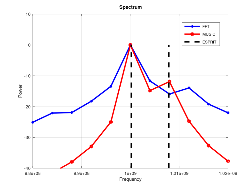
In this post we discuss two of the most popular subspace methods of frequency estimation namely MUSIC* and ESPRIT**. As a reference FFT method is also presented. Both MUSIC and ESPRIT work by separating the noisy signal into signal subspace and noise subspace. MUSIC works by exploiting the fact that noise eigen vectors that compose the noise subspace are orthogonal to the signal vectors (or steering vectors). So, we can search for the signal vectors that are most orthogonal to the noise eigen vectors and that gives us a frequency estimate. MUSIC is in fact an advanced form of Pisarenko Harmonic Decomposition (PHD) where the model order is one more than the number of sinusoids. There is no such limitation in MUSIC.
Unlike MUSIC which exploits the noise subspace, ESPRIT method uses the signal subspace. It estimates the signal subspace S from the estimate of the signal correlation matrix R (same correlation matrix that was used to estimate noise subspace in MUSIC algorithm). Here is the trick you need to perform on the eigen vectors forming the signal subspace S. Split the matrix S into two staggered matrices S1 and S2 of size (M-1) x p each, where M is the model order and p is the number of sinusoids. S1 is matrix S without the last row and S2 is the matrix S without the first row. Now divide the second matrix S2 by S1 using the Least Squares (LS) approach to obtain matrix P. The angles of eigen values of P give us the estimate of the angular frequency.
It is seen that frequency resolution of FFT and MUSIC methods depends upon the size of the temporal window. Greater the length of the time window higher is the frequency resolution. In the results we have shown the frequency resolution is 4MHz. But there is no such barrier for the ESPRIT method. In fact, in the absence of noise, we have observed that ESPRIT method can even decipher sinusoids placed 0.1 MHz apart. But once noise is added the frequency estimation of ESPRIT is not that great. So, for this method the limiting factor is the AWGN noise added to the signal not the size of the temporal window. Lastly, for the simulation scenario we have considered the model size M for MUSIC and ESPRIT is set to 100. We would further investigate this in a future post.

%%%%%%%%%%%%%%%%%%%%%%%%%%%%%%%%%%%%%%%%%
%       SPECTRAL ESTIMATION USING
%      FFT, MUSIC/PISARENKO, ESPRIT
%           www.raymaps.com
%%%%%%%%%%%%%%%%%%%%%%%%%%%%%%%%%%%%%%%%%
clear all
close all

N=1001;             %Number of samples
f1=1.0000e9;        %Frequency of tone 1
f2=1.0200e9;        %Frequency of tone 2
fs=4*f1;            %Sampling frequency
w1=2*pi*f1/fs;      %Angular frequency of tone 1
w2=2*pi*f2/fs;      %Angular frequency of tone 2

%%%%% Signal Generation in AWGN Noise %%%%%
n=0:N-1;
s1=sqrt(1.00)*exp(i*w1*n);
s2=sqrt(0.10)*exp(i*w2*n);
wn=sqrt(0.10)*(randn(1,N)+i*randn(1,N));
x=s1+s2+wn;
x=x(:);

%%%%% FFT Spectrum Generation %%%%%
f=0:fs/(N-1):fs;
FFT_abs=abs(fft(x));
plot(f,20*log10(FFT_abs/max(FFT_abs)),'linewidth',3,'b+-');
hold on

%%%%% MUSIC/Pisarenko Spectrum Generation %%%%%
M=100;
p=2;

f=0:fs/(N-1):fs;
w=2*pi*f/fs;

cov_matrix=zeros(M,M);
for n=1:N-M+1
  cov_matrix=cov_matrix+(x(n:n+M-1))*(x(n:n+M-1))';
end

[V,lambda]=eig(cov_matrix);
e=exp(j*((0:M-1)')*w);

den=zeros(length(w),1);
for n=1:M-p
  v=(V(:,n));
  den=den+(abs((e')*v)).^2;
end
PSD_MUSIC=1./den;
plot(f,10*log10(PSD_MUSIC/max(PSD_MUSIC)),'linewidth',3,'ro-')
hold on

%%%%% ESPRIT Based Frequency Calculation %%%%%
M=100;
p=2;

cov_matrix=zeros(M,M);
for n=1:N-M+1
  cov_matrix=cov_matrix+(x(n:n+M-1))*(x(n:n+M-1))';
end

[U,E,V]=svd(cov_matrix);
S=U(:,1:p);
S1=S(1:M-1,:);
S2=S(2:M,:);
P=S1\S2;
w=angle(eig(P));
f_est=fs*w/(2*pi);

%%%%% Plotting the PSD %%%%%
line([f_est(1), f_est(1)],[-40, 0],'Color','Black','LineStyle','--','linewidth',3);
line([f_est(2), f_est(2)],[-40, 0],'Color','Black','LineStyle','--','linewidth',3);
title('Spectrum')
xlabel('Frequency')
ylabel('Power')
legend('FFT','MUSIC','ESPRIT')
axis([0.98e9 1.04e9 -40 10])
grid on
hold off
Note:
- ESPRIT method can be thought of as differential demodulation of a Continuous Phase Modulated (CPM) signal. But instead of working with staggered samples we are working with staggered matrices. It’s the rotation that want to measure in both.
- One point to be noted is that both MUSIC and ESPRIT methods require the knowledge of number of sinusoids embedded in noise. FFT on the other hand does not need this information beforehand.
- From the code it may seem that noise variance is 0.1 but its actually 0.1 per dimension. The total noise variance is 0.2 resulting in an SNR of 10*log10(1/0.2)=7dB.
- At a Sampling Frequency of 4GHz, 1001 samples translate to a time window of only 250nsec. Thus the resolution of FFT method is 1/250nsec=4MHz.
- Please note that the Zero Crossing algorithm we presented in the last post can be easily modified to work with complex exponentials. After all, a complex exponential can be broken down into a real and imaginary part and Zero Crossings of each can be calculated separately.
*MUSIC: Multiple Signal Classification
**ESPRIT: Estimation of Signal Parameters via Rotational Invariant Techniques
References:
https://en.wikipedia.org/wiki/MUSIC_(algorithm)
https://en.wikipedia.org/wiki/Pisarenko_harmonic_decomposition
https://en.wikipedia.org/wiki/Estimation_of_signal_parameters_via_rotational_invariance_techniques
20 thoughts on “A Comparison of FFT, MUSIC and ESPRIT Methods of Frequency Estimation”
Dear John, in general the amplitude of incident waves are A1, A2,…or A in the equation in vector form but you have assumed the amplitudes as unity which is not necessary.
We have assumed A=1.
Dear john, can we estimate amplitudes of the incident plane waves with the help of MUSIC algorithm? If yes, then how i.e., what changes should we do in the above code for this purpose?
Dear John if we have M sensors, K sources are incident on these M sensors and K is not known while M is known then how will we detect the sources i.e., how will we find K using these algorithms?
There are pretty standard techniques for this…you will have to look up the literature…
This should get you started: https://www.comm.utoronto.ca/~rsadve/Notes/DOA.pdf
I am also doing a post on this.
Dear John you have used theses algorithms for frequency estimation only.
But if we have M sensors, K sources are incident on these M sensors and K is not known while M is known then how will we detect the sources i.e., how will we find K using these algorithms? How will we find power of the noise using these algorithms? Also if we have some interference then how will we suppress that interference?
I suggest you again look at the posts on Uniform Linear Array.
Finding multiple signals in noise is a difficult problem if you do not know how many signals are there. As a starting point use the FFT/DFT to find the spectrum and then define a threshold (like -20dB from the peak). Anything above the threshold is a valid signal.
Hope this helps!
Is this ESPRIT code for detection of frequency? If yes, then what change should I do in it to estimate angles of the two signals?
Detection of frequency and detection of Angle of Arrival (AoA) are similar problems (one has time domain samples other has spatial domain samples). I would let you think about it. Do let me know if you are able to crack it!
Thank you very much for your hints. I will try my best.
Dear John I have a confusion. The confusion is what is the difference between coherent signals and correlated signals? In your above code, you have generated two signals as below:
s1=sqrt(1.00)*exp(i*w1*n);
s2=sqrt(0.10)*exp(i*w2*n);
Now their frequencies are different. So are they coherent signals or correlated signals? If these are coherent signals, then how will we generate correlated signals and vice versa? Further is there any difference between their covariance matrices or their covariance matrices are the same?
The signals are not coherent or correlated.
Thank you very much for your kind response.
Dear John what is meant by coherent signals? If if we have three sources of same frequencies but different phases, are they coherent or not or for coherent signals, their frequencies must be different but phases must be the same. If we have three signals of different frequencies and different directions i.e., 30, 40 and 60. Then how will I estimate these directions using only the given MUSIC algorithm?
1. Coherent signals are aligned in phase and frequency.
2. You can separate signals based on direction of arrival (DoA), frequency may be same or different.
If I have a matrix as below:
S=[ 0.6661 – 0.7458i 0.4210 – 0.9071i 1.0000 + 0.0000i;
-0.9127 + 0.4086i -0.8429 + 0.5381i 1.0000 + 0.0000i;
1.0000 + 0.0000i 1.0000 + 0.0000i 1.0000 + 0.0000i;
-0.9127 – 0.4086i -0.8429 – 0.5381i 1.0000 – 0.0000i;
0.6661 + 0.7458i 0.4210 + 0.9071i 1.0000 – 0.0000i];
Then to find its covariance matrix, we use the Matlab command cov() i.e.,
Rmm=cov(S);
Likewise if we don’t want to use the built-in cov() command, then we normally find the covariance matrix of S as below:
Rmm= S*S’/length(S(1,:));
Now when I find the covariance matrices using these two methods, I get Rmm whose size is different in each case i.e., in 1st method I get Rmm whose size is 3×3 but in 2nd method I get Rmm whose size is 5×5. So why is this difference in sizes and how will we know that which command we should use?
Try S’*S, it will fix the dimensions.
Thank you very much dear John for your response.
Dear John you have used theses algorithms for frequency estimation only.
But if we have M sensors, K sources are incident on these M sensors and K is not known while M is known then how will we detect the sources i.e., how will we find K using these algorithms? How will we find power of the noise using these algorithms? Also if we have some interference then how will we suppress that interference?