The Shannon Capacity of a channel is the data rate that can be achieved over a given bandwidth (BW) and at a particular signal to noise ratio (SNR) with diminishing bit error rate (BER). This has been discussed in an earlier post for the case of SISO channel and additive white Gaussian noise (AWGN). For a MIMO fading channel the capacity with channel not known to the transmitter is given as (both sides have been normalized by the bandwidth [1]):
Shannon Capacity of a MIMO Channel
where NT is the number of transmit antennas, NR is the number of receive antennas, γ is the signal to interference plus noise ratio (SINR), INR is the NRxNR identity matrix and H is the NRxNT channel matrix. Furthermore, hij, an element of the matrix H defines the complex channel coefficient between the ith receive antenna and jth transmit antenna. It is quite obvious that the channel capacity (in bits/sec/Hz) is highly dependent on the structure of matrix H. Let us explore the effect of H on the channel capacity.
Let us first consider a 4×4 case (NT=4, NR=4) where the channel is a simple AWGN channel and there is no fading. For this case hij=1 for all values of i and j. It is found that channel capacity of this simple channel for an SINR of 10 dB is 5.36bits/sec/Hz. It is further observed that the channel capacity does not change with number of transmit antennas and increases logarithmically with increase in number of receive antennas. Thus it can be concluded that in an AWGN channel no multiplexing gain is obtained by increasing the number of transmit antennas.
We next consider a more realistic scenario where the channel coefficients hij are complex with real and imaginary parts having a Gaussian distribution with zero mean and variance 0.5. Since the channel H is random the capacity is also a random variable with a certain distribution. An important metric to quantify the capacity of such a channel is the Complimentary Cumulative Distribution Function (CCDF). This curve basically gives the probability that the MIMO capacity is above a certain threshold.
Complimentary Cumulative Distribution Function of Capacity
It is obvious (see figure above) that there is a very high probability that the capacity obtained for the MIMO channel is significantly higher than that obtained for an AWGN channel e.g. for an SINR of 9 dB there is 90% probability that the capacity is greater than 8 bps/Hz. Similarly for an SINR of 12 dB there is a 90% probability that the capacity is greater than 11 bps/Hz. For a stricter threshold of 99% the above capacities are reduced to 7.2 bps/Hz and 9.6 bps/Hz.
In a practical system the channel coefficients hij would have some correlation which would depend upon the antenna spacing. Lower the antenna spacing higher would be the antenna correlation and lower would be the MIMO system capacity. This would be discussed in a future post.
The MATLAB code for calculating the CCDF of channel capacity of a MIMO channel is given below.
clear all
close all

Nr=4;
Nt=4;
I=eye(Nr);
g=15.8489;

for n=1:10000
    H=sqrt(1/2)*randn(Nr,Nt)+j*sqrt(1/2)*randn(Nr,Nt);
    C(n)=log2(det(I+(g/Nt)*(H*H')));
end

[a,b]=hist(real(C),100);
a=a/sum(a);
plot(b,1-cumsum(a));
xlabel('Capacity (bps/Hz)')
ylabel('Probability (Capacity > Abcissa)')
grid on
[1] G. J. Foschini and M. J. Gans,”On limits of Wireless Communications in a Fading Environment when Using Multiple Antennas”, Wireless Personal Communications 6, pp 311-335, 1998.
We had previously presented a method of generating a temporally correlated Rayleigh fading sequence. This was based on Smith’s fading simulator which was based on Clark and Gan’s fading model. We now present a highly efficient method of generating a correlated Rayleigh fading sequence, which has been adapted from Young and Beaulieu’s technique [1]. The architecture of this fading simulator is shown below.
Modified Young’s Fading Simulator
This method essentially involves five steps.
1. Generate two Gaussian random sequences of length N each.
2. Multiply these sequences by the square root of Doppler Spectrum S=1.5./(pi*fm*sqrt(1-(f/fm).^2).
3. Add the two sequences in quadrature with each other to generate a length N complex sequence (we have added the two sequences before multiplying with the square root of Doppler Spectrum in our simulation).
4. Take the M point complex inverse DFT where M=(fs/Δf)+1.
5. The absolute value of the resulting sequence defines the envelope of the Rayleigh faded signal with the desired temporal correlation (based upon the Doppler frequency fm).
A point to be noted here is that although the Doppler spectrum is defined from -fm to +fm the IDFT has to be taken from -fs/2 to +fs/2. This is achieved by stuffing zeros in the vacant frequency bins from -fs/2 to +fs/2. The MATLAB code for this simulator is given below.
%%%%%%%%%%%%%%%%%%%%%%%%%%%%%%%%%%%%%%%%%%%%%%%%%%%%%%%%%%%%%%%%%%%%%%%%%%
% RAYLEIGH FADING SIMULATOR BASED UPON YOUNG'S METHOD
% N is the number of paths
% M is the total number of points in the frequency domain
% fm is the Doppler frequency in Hz
% fs is the sampling frequency in Hz
% df is the step size in the frequency domain
% Copyright RAYmaps (www.raymaps.com)
%%%%%%%%%%%%%%%%%%%%%%%%%%%%%%%%%%%%%%%%%%%%%%%%%%%%%%%%%%%%%%%%%%%%%%%%%%
clear all;
close all;

N=64;
fm=70;
df=(2*fm)/(N-1);
fs=7.68e6;
M=round(fs/df);
T=1/df;
Ts=1/fs;

% Generate 2xN IID zero mean Gaussian variates
g1=randn(1,N);
g2=randn(1,N);
g=g1-j*g2;

% Generate Doppler Spectrum
f=-fm:df:fm;
S=1.5./(pi*fm*sqrt(1-(f/fm).^2));
S(1)=2*S(2)-S(3);
S(end)=2*S(end-1)-S(end-2);

% Multiply square root of Doppler Spectrum with Gaussian random sequence
X=g.*sqrt(S);

% Take IFFT
F_zero=zeros(1, round((M-N)/2));
X=[F_zero, X, F_zero];
x=ifft(X,M);
r=abs(x);
r=r/mean(r);

% Plot the Rayleigh envelope
t=0:Ts:T-Ts;
plot(t,10*log10(r))
xlabel('Time(sec)')
ylabel('Signal Amplitude (dB)')
%%%%%%%%%%%%%%%%%%%%%%%%%%%%%%%%%%%%%%%%%%%%%%%%%%%%%%%%%%%%%%%%%%%%%%%%%%
The question now is that how do we verify that the generated Rayleigh fading sequence has the desired statistical properties. This can be verified by looking at the level crossing rate (LCR) and average fade duration (AFD) of the generated sequence as well as the PDF and Autocorrelation function. The LCR and AFD calculated for N=64 and fm=70 Hz and threshold of -10 dB (relative to the average signal power) is given below.
LCR
Simulation: 15.55
Theoretical: 15.46
AFD
Simulation: 453 usec
Theoretical: 508 usec
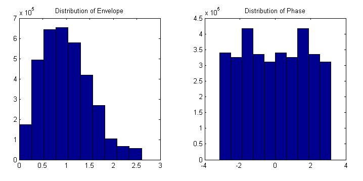
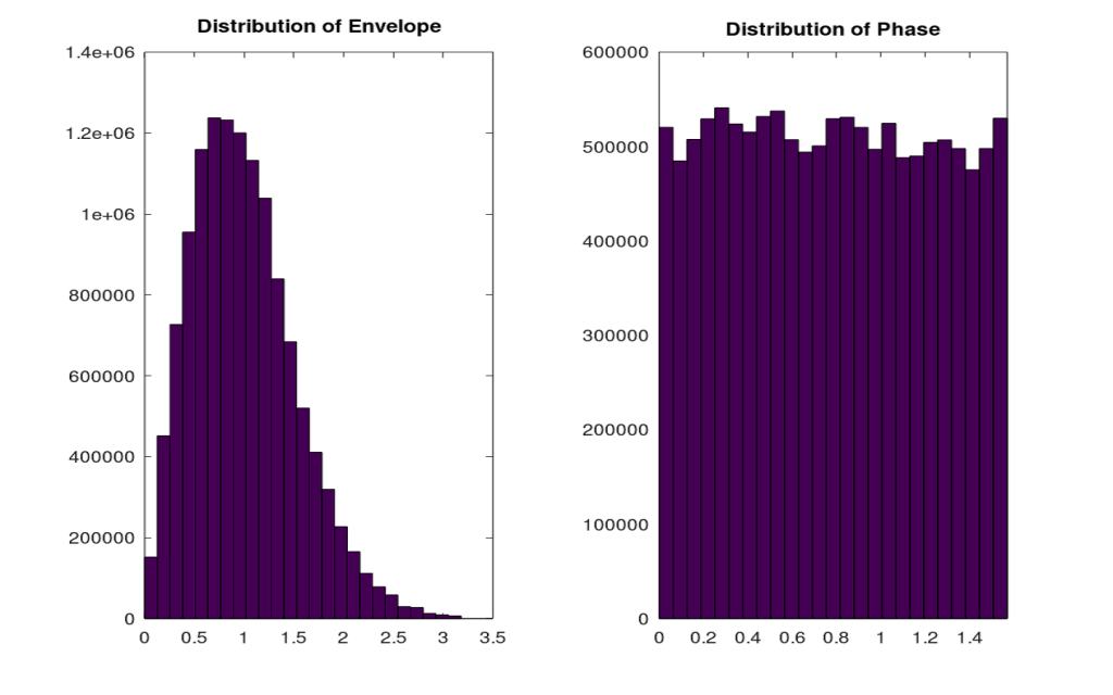
It is observed that the theoretical and simulation results for the LCR and AFD match reasonably well. We next examine the distribution of the envelope and phase of the resulting sequence x. It is found that the envelope of x is Rayleigh distributed while the phase is uniformly distributed from -pi to pi. This is shown in the figure below. So we are reasonably satisfied that our generated sequence has the desired statistical properties.
Envelope and Phase Distribution for fm=70Hz
Rayleigh Fading Simulator Based on Young’s Filter
In the above simulation of Rayleigh fading sequence we reduced the computation load of Smith’s simulator by reducing the IFFT operations on two branches to a single IFFT operation. However, we still used the Doppler spectrum proposed by Smith. Now we use the filter with spectrum Fk defined by Young in [1]. The code for this is given below.
%%%%%%%%%%%%%%%%%%%%%%%%%%%%%%%%%%%%%%%%%%%%%%%%%%%%%%%%%%%%%%%%%%%%%%%%%%
% RAYLEIGH FADING SIMULATOR BASED UPON YOUNG'S METHOD
% N is the number of points in the frequency domain
% fm is the Doppler frequency in Hz
% fs is the sampling frequency in Hz
% Copyright RAYmaps (www.raymaps.com)
%%%%%%%%%%%%%%%%%%%%%%%%%%%%%%%%%%%%%%%%%%%%%%%%%%%%%%%%%%%%%%%%%%%%%%%%%%
clear all;
close all;

N=2^20;
fm=300;
fs=7.68e6;
Ts=1/fs;

% Generate 2xN IID zero mean Gaussian variates
g1=randn(1,N);
g2=randn(1,N);
g=g1-j*g2;

% Generate filter F
F = zeros(1,N);
dopplerRatio = fm/fs;
km=floor(dopplerRatio*N);
for k=1:N
if k==1,
F(k)=0;
elseif k>=2 && k<=km,
F(k)=sqrt(1/(2*sqrt(1-((k-1)/(N*dopplerRatio))^2)));
elseif k==km+1,
F(k)=sqrt(km/2*(pi/2-atan((km-1)/sqrt(2*km-1))));
elseif k>=km+2 && k<=N-km,
F(k) = 0;
elseif k==N-km+1,
F(k)=sqrt(km/2*(pi/2-atan((km-1)/sqrt(2*km-1))));
else
F(k)=sqrt(1/(2*sqrt(1-((N-(k-1))/(N*dopplerRatio))^2)));
end
end

% Multiply F with Gaussian random sequence
X=g.*F;

% Take IFFT
x=ifft(X,N);
r=abs(x);
r=r/mean(r);

% Plot the Rayleigh envelope
T=length(r)*Ts;
t=0:Ts:T-Ts;
plot(t,10*log10(r))
xlabel('Time(sec)')
ylabel('Signal Amplitude (dB)')
axis([0 0.05 -15 5])
%%%%%%%%%%%%%%%%%%%%%%%%%%%%%%%%%%%%%%%%%%%%%%%%%%%%%%%%%%%%%%%%%%%%%%%%%%
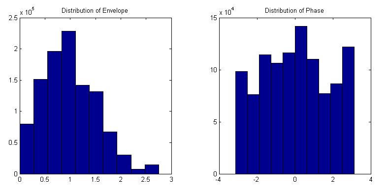
The above code was used to generate Rayleigh sequences of varying lengths with Doppler frequencies of 5 Hz, 70 Hz and 300 Hz. The sampling frequency was fixed at 7.68 MHz (corresponding to a BW of 5 MHz). It must be noted that in this simulation the length of the Gaussian sequence is equal to the filter length in the frequency domain. It was found that to generate a Rayleigh sequence of reasonable length the length of the Gaussian sequence has to be quite large (2^20 in the above example). As before we calculated the distribution of envelope and phase of the generated sequence as well as the LCR and AFD. These were found to be within reasonable margins.
Envelope Phase Distribution at fm=300 Hz
Note:
1. Level crossing rate (LCR) is defined as number of times per second the signal envelope crosses a given threshold. This could be either in the positive direction or negative direction.
2. Average fade duration (AFD) is the average duration that the signal envelope remains below a given threshold once it crosses that threshold. Simply it is the average duration of a fading event.
3. The LCR and AFD are interconnected and the product of these two quantities is a constant.
[1] David J. Young and Norman C. Beaulieu, "The Generation of Correlated Rayleigh Random Variates by Inverse Discrete Fourier Transform", IEEE Transactions on Communications vol. 48 no. 7 July 2000.
Just to recap, building an LTE fading simulator with the desired temporal and spatial correlation is a three step procedure.
1. Generate Rayleigh fading sequences using Smith’s method which is based on Clarke and Gan’s fading model.
2. Introduce spatial correlation based upon the spatial correlation matrices defined in 3GPP 36.101.
3. Use these spatially and temporally correlated sequences as the filter taps for the LTE channel models.
We have already discussed step 1 and 3 in our previous posts. We now focus on step 2, generating spatially correlated channels coefficients.
3GPP has defined spatial correlation matrices for the Node-B and the UE. These are defined for 1,2 and 4 transmit and receive antennas. These are reproduced below.
Spatial Correlation Matrix
The parameters ‘alpha’ and ‘beta’ are defined as:
Low Correlation
alpha=0, beta=0
Medium Correlation
alpha=0.3, beta=0.9
High Correlation
alpha=0.9, beta=0.9
The combined effect of antenna correlation at the transmitter and receiver is obtained by taking the Kronecker product of individual correlation matrices e.g. for a 2×2 case the correlation matrix is given as:
Correlation Matrix for 2×2 MIMO
Multiplying the square root of the correlation matrix with the vector of channel coefficients is equivalent to taking a weighted average e.g. for the channel between transmit antenna 1 and receive antenna 1 the correlated channel coefficient h11corr is given as:
h11corr=w1*h11+w2*h12+w3*h21+w4*h22
where w1=1 and w2, w3 and w4 are less than one and greater than zero. For the high correlation case described above the channel coefficient is calculated as:
From a practical point of antenna correlation is dependent on the antenna separation. Greater the antenna spacing lower is the antenna correlation and better the system performance. However, a base station requires much higher antenna spacing than a UE to achieve the same level of antenna correlation. This is due to the fact the base station antennas are placed much higher than a UE. Therefore the signals arriving at the base station are usually confined to smaller angles and experience similar fading. A UE on the other hand has a lot of obstacles in the surrounding areas which results in higher angle spread and uncorrelated fading between the different paths.
As discussed previously building an LTE fading simulator is a three step procedure.
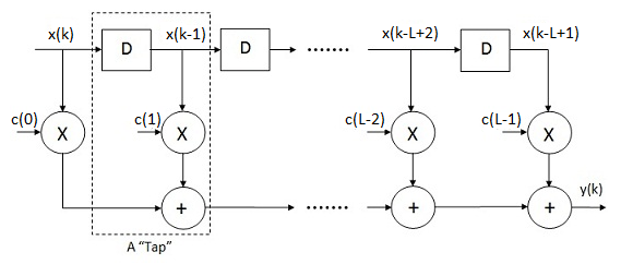
1. Generate a temporally correlated Rayleigh fading sequence. This step would be repeated for each channel tap and transmit receive antenna combination e.g. for a 2×2 MIMO system and EPA channel model with 7 taps the number of fading sequences to be generated is 4×7=28. The temporal correlation of these fading sequences is controlled by the Doppler frequency. A higher Doppler frequency results in faster channel variations and vice versa.
2. Introduce spatial correlation between the parallel paths e.g. for a 2×2 MIMO system a 4×4 antenna corelation matrix would be used to introduce spatial correlation between the 4 parallel paths h11, h12, h21 and h22. This can be thought of as a weighted average. A channel coefficient between Tx-1 and Rx-1 would be calculated as h11=w1*h11+w2*h12+w3*h21+w4*h22. In this case the weight ‘w1’ would have a value of 1 whereas the other weights would have a value less than 1. If w2=w3=w4=0 there is no correlation between h11 and other channel coefficients.
2-Transmit 2-Receive Channel Model
3. Once the sequences with the desired temporal and spatial correlation have been generated their mean power would have to be adjusted according to the power delay profile of the selected channel model (EPA, EVA or ETU). The number of channel coefficients increases exponentially with the number of transmit and receiver antennas e.g. for a 4×4 MIMO system each filter tap would have to be calculated after performing a weighted average of 16 different channel taps. And this step would have to be repeated for each filter tap resulting in a total of 16×7=112 fading sequences.
Since the wireless channel is time varying the channel taps c(0) c(1)…..c(L-1) are also time varying with either Rayleigh or Rician distribution. It is quite easy to generate Rayleigh random variables with the desired power and distribution, however, when these Rayleigh random variables are required to have temporal correlation the process becomes a bit complicated. Temporal correlation of these variables depends upon the Doppler frequency which is turn depends upon the speed of the mobile device. The Doppler frequency is defined as:
fd=v*cos(theta)/lambda
where
fd is the Doppler Frequency in Hz v is the receiver velocity in m/sec lambda is the wavelength in m and theta is the angle between the direction of arrival of the signal and the direction of motion
A simple method for generating Rayleigh random variables with the desired temporal correlation was devised by Smith [1]. His method was based on Clark and Gans fading model and has been widely used in simulation of wireless communication systems.
The method for generating the Rayleigh fading envelope with the desired temporal correlation is given below (modified from Theodore S. Rappaport Text).
1. Define N the number of Gaussian RVs to be generated, fm the Doppler frequency in Hz, fs the sampling frequency in Hz, df the frequency spacing which is calculated as df=(2*fm)/(N-1) and M total number of samples in frequency domain which is calculated as M=(fs/df).
2. Generate two sequences of N/2 complex Gaussian random variables. These correspond to the frequency bins up to fm. Take the complex conjugate of these sequences to generate the N/2 complex Gaussian random variables for the negative frequency bins up to -fm.
3. Multiply the above complex Gaussian sequences g1 and g2 with square root of the Doppler Spectrum S generated from -fm to fm. Calculate the spectrum at -fm and +fm by using linear extrapolation.
4. Extend the above generated spectra from -fs/2 to +fs/2 by stuffing zeros from -fs/2 to -fm and fm to fs/2. Take the IFFT of the resulting spectra X and Y resulting in time domain signals x and y.
5. Add the absolute values of the resulting signals x and y in quadrature. Take the absolute value of this complex signal. This is the desired Rayleigh distributed envelope with the required temporal correlation.
The Matlab code for generating Rayleigh random sequence with a Doppler frequency of fm Hz is given below.
%%%%%%%%%%%%%%%%%%%%%%%%%%%%%%%%%%%%%%%%%%%%%%%%%%%%%%%%%%%%%%%%
% RAYLEIGH FADING SIMULATOR BASED UPON SMITH'S METHOD
% N is the number of paths
% M is the total number of points in the frequency domain
% fm is the Doppler frequency in Hz
% fs is the sampling frequency in Hz
% df is the step size in the frequency domain
% Copyright RAYmaps (www.raymaps.com)
%%%%%%%%%%%%%%%%%%%%%%%%%%%%%%%%%%%%%%%%%%%%%%%%%%%%%%%%%%%%%%%%
clear all;
close all;

N=1000;
fm=300;
df=(2*fm)/(N-1);
fs=7.68e6;
M=round(fs/df);
T=1/df;
Ts=1/fs;

% Generate two sequences of N complex Gaussian random variables
g=randn(1,N/2)+j*randn(1,N/2);
gc=conj(g);
g1=[fliplr(gc), g];

g=randn(1,N/2)+j*randn(1,N/2);
gc=conj(g);
g2=[fliplr(gc), g];

% Generate Doppler Spectrum S
f=-fm:df:fm;
S=1.5./(pi*fm*sqrt(1-(f/fm).^2));
S(1)=2*S(2)-S(3);
S(end)=2*S(end-1)-S(end-2);

% Multiply the sequences with the Doppler Spectrum S, take IFFT
X=g1.*sqrt(S);
X=[zeros(1,round((M-N)/2)), X, zeros(1,round((M-N)/2))];
x=abs(ifft(X,M));

Y=g2.*sqrt(S);
Y=[zeros(1,round((M-N)/2)), Y, zeros(1,round((M-N)/2))];
y=abs(ifft(Y,M));

% Find the resulting Rayleigh faded envelope
z=x+j*y;
r=abs(z);
r=r/sqrt(mean(r.^2));

t=0:Ts:T-Ts;
plot(t,10*log10(r),'r')
xlabel('Time(sec)')
ylabel('Envelope (dB)')
axis([0 0.01 -10 5])
%%%%%%%%%%%%%%%%%%%%%%%%%%%%%%%%%%%%%%%%%%%%%%%%%%%%%%%%%%%%%%%%
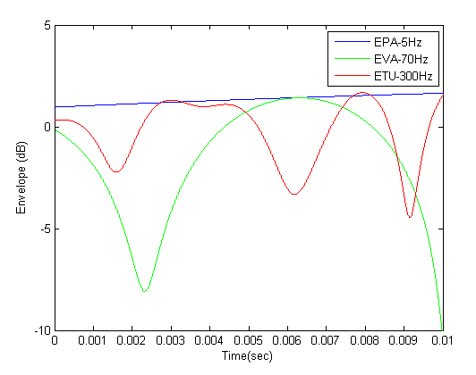
The above code generates a Rayleigh random sequence with samples spaced at 0.1302 usec. This corresponds to a sampling frequency of 7.68 MHz which is the standard sampling frequency for a bandwidth of 5MHz. Similarly, the sampling rate for 10 MHz and 20 MHz is 15.36 MHz and 30.72 MHz respectively. The Doppler frequency can also be changed according to the scenario. LTE standard defines 3 channel models EPA, EVA and ETU with Doppler frequencies of 5 Hz, 70 Hz and 300 Hz respectively. These are also known as Low Doppler, Medium Doppler and High Doppler respectively.
The above code generated Rayleigh sequences of varying lengths for the three cases. But in all the cases it is in excess of 10 msec and can be used as the fading sequence for an LTE frame. Just to recall an LTE frame is of 10 msec duration with 20 time slots of 0.5 msec each. If each slot contains 7 OFDM symbols the total length of a fading sequence is 140 symbols.
Rayleigh Fading Envelope and Phase Distribution
It is seen that the fluctuation in the channel increases with Doppler frequency. The channel is almost static for a Doppler frequency of 5 Hz and varies quite rapidly for a Doppler frequency of 300 Hz. It is also shown above that the envelope of z is Rayleigh distributed and phase of z is Uniformly distributed. However, the range of phase is from 0 to pi/2. This needs to be further investigated. The level crossing rate and average fade duration can also be measured.
This is the process for generating one Rayleigh distributed channel tap. This step would have to be repeated for the number of taps in the channel model which could be 7 or 9 for the LTE channel models. A Ricean distributed channel tap can be generated in a similar fashion. MIMO channel taps can also be generated using the above described method, however, we would need to understand the concept of antenna correlation before we do that.
Level Crossing Rate and Average Fade Duration
Level crossing rate (LCR) is defined as number of times per second the signal envelope crosses a given threshold. This could be either in the positive direction or negative direction. Average fade duration (AFD) is the average duration that the signal envelope remains below a given threshold once it crosses that threshold. Simply it is the average duration of a fading event. The LCR and AFD are interconnected and the product of these two quantities is a constant. The program given below calculates the LCR and AFD of the above generated envelope r.
The program calculates both the simulated and theoretical values of LCR and AFD e.g. for a threshold level of 0.3 (-5.22 dB) the LCR and AFD values calculated for fm=70 Hz and N=32 are:
LCR simulation = 45.16
LCR theoretical = 43.41
AFD simulation = 0.0015 sec
AFD theoretical = 0.0016 sec
It can be seen that the theoretical and simulation results match quite well. This gives us confidence that are generated envelope has the desired statistical characteristics.
%%%%%%%%%%%%%%%%%%%%%%%%%%%%%%%%%%%%%%%%%%%%%%%%%%%%%%
% PROGRAM TO CALCULATE THE LCR and AFD
% Rth: Level to calculate the LCR and AFD
% Rrms: RMS level of the signal r
% rho: Ratio of defined threshold and RMS level
% Copyright RAYmaps (www.raymaps.com)
%%%%%%%%%%%%%%%%%%%%%%%%%%%%%%%%%%%%%%%%%%%%%%%%%%%%%%
Rth=0.30;
Rrms=sqrt(mean(r.^2));
rho=Rth/Rrms;

count1=0;
count2=0;

for n=1:length(r)-1
     if r(n) < Rth && r(n+1) > Rth
        count1=count1+1;
     end
    if r(n) < Rth
        count2=count2+1;
    end
end
LCR=count1/(T)
AFD=((count2*Ts)/T)/LCR

LCR_num=sqrt(2*pi)*fm*rho*exp(-(rho^2))
AFD_num=(exp(rho^2)-1)/(rho*fm*sqrt(2*pi))
%%%%%%%%%%%%%%%%%%%%%%%%%%%%%%%%%%%%%%%%%%%%%%%%%%%%%%
Note:
1. According to Wireless Communications Principles and Practice by Ted Rappaport "Perform an IFFT on the resulting frequency domain signals from the in-phase and quadrature arms to get two N-length time series, and add the squares of each signal point in time to create an N-point time series. Note that each quadrature arm should be a real signal after IFFT". Now this point about the signal being real after IFFT is not always satisfied by the above program. The condition can be satisfied by playing around with the value of N a bit.
2. Also, we take the absolute value of both the time series after IFFT operation to make sure that we get a real valued sequence. However, taking the absolute value of both the in-phase and quadrature terms makes z fall in the first quadrant and the phase of z to vary from 0 to pi/2. A better approach might be to use the 'real' function instead of 'abs' function so that the phase can vary from 0 to 2pi.
3. A computationally efficient method of generating Rayleigh fading sequence is given here.
[1] John I. Smith, "A Computer Generated Multipath Fading Simulation for Mobile Radio", IEEE Transactions on Vehicular Technology, vol VT-24, No. 3, August 1975.