Tag Archives: BER

M-QAM Bit Error Rate in Rayleigh Fading

May 22, 2012BER Performance, Fundamentals, LTE, Modulation, WiMAXBER, Fading, Modulation, QAM, Rayleigh FadingYasir Ahmed (aka John)

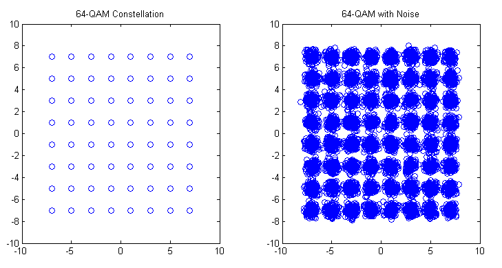
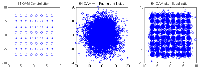
We have previously discussed the bit error rate (BER) performance of M-QAM in AWGN. We now discuss the BER performance of M-QAM in Rayleigh fading. The one-tap Rayleigh fading channel is generated from two orthogonal Gaussian random variables with variance of 0.5 each. The complex random channel coefficient so generated has an amplitude which is Rayleigh distributed and a phase which is uniformly distributed. As usual the fading channel introduces a multiplicative effect whereas the AWGN is additive.

The function “QAM_fading” has three inputs, ‘n_bits’, ‘M’, ‘EbNodB’ and one output ‘ber’. The inputs are the number of bits to be passed through the channel, the alphabet size and the Energy per Bit to Noise Power Spectral Density in dB respectively whereas the output is the bit error rate (BER).

%%%%%%%%%%%%%%%%%%%%%%%%%%%%%%%%%%%%%%%%%%%%%%%%%%%%%%%%%%%%%%%%%%
% FUNCTION THAT CALCULATES THE BER OF M-QAM IN RAYLEIGH FADING
% n_bits: Input, number of bits
% M: Input, constellation size
% EbNodB: Input, energy per bit to noise power spectral density
% ber: Output, bit error rate
% Copyright RAYmaps (www.raymaps.com)
%%%%%%%%%%%%%%%%%%%%%%%%%%%%%%%%%%%%%%%%%%%%%%%%%%%%%%%%%%%%%%%%%%
function[ber]= QAM_fading(n_bits, M, EbNodB)
% Transmitter
k=log2(M);
EbNo=10^(EbNodB/10);
x=transpose(round(rand(1,n_bits)));
h1=modem.qammod(M);
h1.inputtype='bit';
h1.symbolorder='gray';
y=modulate(h1,x);

% Channel
Eb=mean((abs(y)).^2)/k;
sigma=sqrt(Eb/(2*EbNo));
w=sigma*(randn(n_bits/k,1)+1i*randn(n_bits/k,1));
h=(1/sqrt(2))*(randn(n_bits/k,1)+1i*randn(n_bits/k,1));
r=h.*y+w;

% Receiver
r=r./h;
h2=modem.qamdemod(M);
h2.outputtype='bit';
h2.symbolorder='gray';
h2.decisiontype='hard decision';
z=demodulate(h2,r);
ber=(n_bits-sum(x==z))/n_bits
return
%%%%%%%%%%%%%%%%%%%%%%%%%%%%%%%%%%%%%%%%%%%%%%%%%%%%%%%%%%%%%%%%%%

The bit error rates of four modulation schemes 4-QAM, 16-QAM, 64-QAM and 256-QAM are shown in the figure above. All modulation schemes use Gray coding which gives a few dB of margin in the BER performance. As with the AWGN case each additional bit per symbol requires about 1.5-2 dB in signal to ratio to achieve the same BER.

Although not shown here similar behavior is observed for higher order modulation schemes such as 1024-QAM and 4096-QAM (the gap in the signal to noise ratio for the same BER is increased to about 5dB).

Lastly we explain some of the terms used above.

Rayleigh Fading

Rayleigh Fading is a commonly used term in simulation of Digital Communication Systems but it tends to differ in meaning in different contexts. The term Rayleigh Fading as used above means a single tap channel that varies from one symbol to the next. It has an amplitude which is Rayleigh distributed and a phase which is Uniformly distributed. A single tap channel means that it does not introduce any Inter Symbol Interference (ISI). Such a channel is also referred to as a Flat Fading Channel. The channel can also be referred to as a Fast Fading Channel since each symbol experiences a new channel state which is independent of its previous state (also termed as uncorrelated).

Gray Coding

When using QAM modulation, each QAM symbol represents 2,3,4 or higher number of bits. That means that when a symbol error occurs a number of bits are reversed. Now a good way to do the bit-to-symbol assignment is to do it in a way such that no neighboring symbols differ by more than one bit e.g. in 16-QAM, a symbol that represents a binary word 1101 is surrounded by four symbols representing 0101, 1100, 1001 and 1111. So if a symbol error is made, only one bit would be in error. However, one must note that this is true only in good signal conditions. When the SNR is low (noise has a higher magnitude) the symbol might be displaced to a location that is not adjacent and we might get higher number of bits in error.

Hard Decision

The concept of hard decision decoding is important when talking about channel coding, which we have not used in the above simulation. However, we will briefly explain it here. Hard decision is based on what is called “Hamming Distance” whereas soft decision is based on what it called “Euclidean Distance”. Hamming Distance is the distance of a code word in binary form, such as 011 differs from 010 and 001 by 1. Whereas the Euclidean distance is the distance before a decision is made that a bit is zero or one. So if the received sequence is 0.1 0.6 0.7 we get a Euclidean distance of 0.8124 from 010 and 0.6782 from 001. So we cannot make a hard decision about which sequence was transmitted based on the received sequence of 011. But based on the soft metrics we can make a decision that 001 was the most likely sequence that was transmitted (assuming that 010 and 001 were the only possible transmitted sequences).

M-QAM Bit Error Rate in AWGN

May 21, 2012BER Performance, Fundamentals, LTE, Modulation, WiMAXAWGN, BER, QAMYasir Ahmed (aka John)

Quadrature Amplitude Modulation has been adopted by most wireless communication standards such as WiMAX and LTE. It provides higher bit rates and consequently higher spectral efficiencies. It is usually used in conjunction with Orthogonal Frequency Division Multiplexing (OFDM) which provides a simple technique to overcome the time varying frequency selective channel.

We have previously discussed the formula for calculating the bit error rate (BER) of QAM in AWGN. We now calculate the same using a simple Monte Carlo Simulation.

%%%%%%%%%%%%%%%%%%%%%%%%%%%%%%%%%%%%%%%%%%%%%%%%%%%%%%%%%%%%%%%%%%
% FUNCTION THAT CALCULATES THE BER OF M-QAM IN AWGN
% n_bits: Input, number of bits
% M: Input, constellation size
% EbNodB: Input, energy per bit to noise power spectral density
% ber: Output, bit error rate
% Copyright RAYmaps (www.raymaps.com)
%%%%%%%%%%%%%%%%%%%%%%%%%%%%%%%%%%%%%%%%%%%%%%%%%%%%%%%%%%%%%%%%%%

function[ber]= QAM_AWGN(n_bits, M, EbNodB)

% Transmitter
k=log2(M);
EbNo=10^(EbNodB/10);
x=transpose(round(rand(1,n_bits)));
h1=modem.qammod(M);
h1.inputtype='bit';
h1.symbolorder='gray';
y=modulate(h1,x);

% Channel
Eb=mean((abs(y)).^2)/k;
sigma=sqrt(Eb/(2*EbNo));
w=sigma*(randn(1,n_bits/k)+1i*randn(1,n_bits/k));
r=y+w';

% Receiver
h2=modem.qamdemod(M);
h2.outputtype='bit';
h2.symbolorder='gray';
h2.decisiontype='hard decision';
z=demodulate(h2,r);
ber=(n_bits-sum(x==z))/n_bits
return
%%%%%%%%%%%%%%%%%%%%%%%%%%%%%%%%%%%%%%%%%%%%%%%%%%%%%%%%%%%%%%%%%%

The above function basically has three inputs and one output. The inputs are the number of bits to be passed through the channel, the size of the constellation and the signal to noise ratio in dB. The output is the bit error rate (BER). The simulation can be divided into three section namely the transmitter, the channel and the receiver. In this simulation we have used Gray coding which gives us about a dB of improvement at low to medium signal to noise ratio.

As seen above the BER obtained through our simulation matches quite well with the BER obtained through the theoretical formula. Each additional bit per symbol required about 2dB extra in signal to noise ratio to achieve the same bit error rate.

Lastly we explain some of the terms used above.

AWGN

All wireless receivers suffer from thermal noise which is a function of absolute temperature and bandwidth of the receiver. This noise is added to the received signal and makes detection of weak signals a major challenge. Just to given you an idea typical GSM receivers have a noise floor of -113 dBm. Therefore, if the received signal has a power of -100 dBm we get a signal to noise ratio (SNR) of 13 dB. In simulation this noise is usually modeled as a Gaussian Random Process. It is additive, as opposed to channel impairments which are multiplicative and has a flat spectrum (thus called White Noise).

Gray Coding

Hard Decision

QAM Theoretical BER in AWGN

December 8, 2011BER Performance, LTE, WiMAX4G, AWGN, BER, LTE, QAM, QPSK, WiMAXYasir Ahmed (aka John)

Quadrature Amplitude Modulation (QAM) is an important modulation scheme as it allows for higher data rates and spectral efficiencies. The bit error rate (BER) of QAM can be calculated through Monte Carlo simulations. However this becomes quite complex as the constellation size of the modulation schemes increases. Therefore a theoretical approach is sometimes preferred. The BER for Gray coded QAM, for even number of bits per symbol, is shown below.

BER of 4-QAM, 16-QAM, 64-QAM, 256-QAM in AWGN

Gray coding ensures that a symbol error results in a single bit error. The code for calculating the theoretical QAM BER for k even (even number of bits per symbol) is given below. The formula for calculating the BER for k odd is different, however, the formula given below can be used a first estimate.

EbNodB=-6:2:24
EbNo=10.^(EbNodB/10);
k=8;
M=2^k;
x=sqrt(3*k*EbNo/(M-1));
Pb=(4/k)*(1-1/sqrt(M))*(1/2)*erfc(x/sqrt(2));
semilogy(EbNodB,Pb)

Note:
1. Each additional bit/symbol requires about 2dB extra in SNR to achieve the same BER.
2. 4-QAM is essentially QPSK modulation.

BER of 64-QAM OFDM in Frequency Selective Fading-II

September 9, 20115G, BER Performance, LTE, Modulation, WiMAXBER, BIT ERROR RATE, LTE, OFDM, QAMYasir Ahmed (aka John)

In the previous post we had considered a static frequency-selective channel. We now consider a time-varying frequency selective channel with 7 taps. Each tap of the time domain filter has a Gaussian distributed real component with variance 1/(2*n_tap) and a Gaussian distributed imaginary component with variance 1/(2*n_tap). The amplitude of each tap is thus Rayleigh distributed and the phase is Uniformly distributed. Since the power in each component is normalized by the filter length (n_tap) the BER performance would remain the same even if the filter length is changed (this has been verified experimentally).

%%%%%%%%%%%%%%%%%%%%%%%%%%%%%%%%%%%%%%%%%%%%%%%%%%%%%%%%%%%%%%%%%%%%%%%%%
% FUNCTION TO SIMULATE PERFORMANCE OF 64-OFDM IN TIME VARYING FREQUENCY SELECTIVE CHANNEL
% n_bits: Input, length of binary sequence
% n_fft: Input, length of FFT (Fast Fourier Transform)
% EbNodB: Input, energy per bit to noise power spectral density ratio
% ber: Output, bit error rate
% Copyright RAYmaps (www.raymaps.com)
%%%%%%%%%%%%%%%%%%%%%%%%%%%%%%%%%%%%%%%%%%%%%%%%%%%%%%%%%%%%%%%%%%%%%%%%%
function[ber]= M_QAM_OFDM_fading(n_bits,n_fft,EbNodB)

Eb=7;
M=64;
k=log2(M);
n_cyc=32;
EbNo=10^(EbNodB/10);
x=transpose(round(rand(1,n_bits)));
h1=modem.qammod(M);
h1.inputtype='bit';
h1.symbolorder='gray';
y=modulate(h1,x);
n_sym=length(y)/n_fft;
n_tap=7;

for n=1:n_sym;
    s_ofdm=sqrt(n_fft)*ifft(y((n-1)*n_fft+1:n*n_fft),n_fft);
    s_ofdm_cyc=[s_ofdm(n_fft-n_cyc+1:n_fft); s_ofdm];
    ht=(1/sqrt(2))*(1/sqrt(n_tap))*(randn(1,n_tap)+j*randn(1,n_tap));
    Hf=fft(ht,n_fft);
    r_ofdm_cyc=conv(s_ofdm_cyc,ht);
    r_ofdm_cyc=(r_ofdm_cyc(1:n_fft+n_cyc));
    wn=sqrt((n_fft+n_cyc)/n_fft)*(randn(1,n_fft+n_cyc)+j*randn(1,n_fft+n_cyc));
    r_ofdm_cyc=r_ofdm_cyc+sqrt(Eb/(2*EbNo))*wn.';
    r_ofdm=r_ofdm_cyc(n_cyc+1:n_fft+n_cyc);
    s_est((n-1)*n_fft+1:n*n_fft)=(fft(r_ofdm,n_fft)/sqrt(n_fft))./Hf.';
end

h2=modem.qamdemod(M);
h2.outputtype='bit';
h2.symbolorder='gray';
h2.decisiontype='hard decision';
z=demodulate(h2,s_est.');
ber=(n_bits-sum(x==z))/n_bits
return
%%%%%%%%%%%%%%%%%%%%%%%%%%%%%%%%%%%%%%%%%%%%%%%%%%%%%%%%%%%%%%%%%%%%%%%%%

As before we have used an FFT size of 128 and cyclic prefix of 32 samples. The FFT and IIFT operations are normalized to maintain the signal to noise ratio (SNR). The extra energy transmitted in the cyclic prefix is also accounted for in the SNR calibration.

64-QAM BER in Time Varying Frequency Selective Channel

It is observed that the BER performance of 64-QAM OFDM in the time-varying frequency-selective channel is quite similar to that in the static frequency-selective channel with complex filter taps. It must be noted that with 64-QAM the goal is to achieve higher bit rate, error rates can be improved using antenna diversity and channel coding schemes.

Given below is the wrapper that should be used along with the above code. The wrapper basically calls the above routine for each value of EbNodB. The length of the binary sequence and the FFT size are other inputs to the function. The bit error rate at the specific EbNodB is the output of the function.

%%%%%%%%%%%%%%%%%%%%%%%%%%%%%%%%%%%
clear all;
close all;
k=6;
n_fft=128;
l=k*n_fft*1e3;
EbNodB=0:2:20;
for n=1:length(EbNodB);n
ber(n)=M_QAM_OFDM_fading(l,n_fft,EbNodB(n));
end;
semilogy(EbNodB,ber,'O-');
grid on
xlabel('EbNo')
ylabel('BER')
%%%%%%%%%%%%%%%%%%%%%%%%%%%%%%%%%%%

In future we would use the standard LTE channel models, namely EPA, EVA and ETU in our simulation.

BER of 64-QAM OFDM in Frequency Selective Fading

September 3, 20115G, BER Performance, LTE, Modulation, WiMAXBER, LTEYasir Ahmed (aka John)

The real benefits of OFDM become apparent in a frequency selective channel. The introduction of the cyclic prefix (guard period) allows us to remove the Intersymbol Interference (ISI) in the time domain and frequency domain equalization allows us to overcome the channel variations in the frequency domain.

We consider a simple FIR filter for our channel model with coefficients ht=[0.8 0.54 0.24 0.10 0.04]. This is a simplistic approach since the channel coefficients are all real which means that all multipath components are co-phase. To model a more realistic channel we then introduce a uniform phase shift to all the channel coefficients.

We use an FFT size of 128 and cyclic prefix of 32 samples (16.67usec) in the simulation given below.

%%%%%%%%%%%%%%%%%%%%%%%%%%%%%%%%%%%%%%%%%%%%%%%%%%%%%%%%%%%%%%%%%%%%%%%%%
% FUNCTION TO SIMULATE THE PERFORMANCE OF 64-QAM OFDM IN STATIC FREQUENCY SELECTIVE CHANNEL
% n_bits: Input, length of binary sequence
% n_fft: Input, length of FFT (Fast Fourier Transform)
% EbNodB: Input, energy per bit to noise power spectral density ratio
% ber: Output, bit error rate
% Copyright RAYmaps (www.raymaps.com)
%%%%%%%%%%%%%%%%%%%%%%%%%%%%%%%%%%%%%%%%%%%%%%%%%%%%%%%%%%%%%%%%%%%%%%%%%
function[ber]= M_QAM_OFDM_fading(n_bits,n_fft,EbNodB)

Eb=7;
M=64;
k=log2(M);
n_cyc=32;
EbNo=10^(EbNodB/10);
x=transpose(round(rand(1,n_bits)));
h1=modem.qammod(M);
h1.inputtype='bit';
h1.symbolorder='gray';
y=modulate(h1,x);
n_sym=length(y)/n_fft;

for n=1:n_sym;
    s_ofdm=sqrt(n_fft)*ifft(y((n-1)*n_fft+1:n*n_fft),n_fft);
    s_ofdm_cyc=[s_ofdm(n_fft-n_cyc+1:n_fft); s_ofdm];
    ht=[0.8 0.54 0.24 0.10 0.04];
    Hf=fft(ht,n_fft);
    r_ofdm_cyc=conv(s_ofdm_cyc,ht);
    r_ofdm_cyc=(r_ofdm_cyc(1:n_fft+n_cyc));
    wn=sqrt((n_fft+n_cyc)/n_fft)*(randn(1,n_fft+n_cyc)+j*randn(1,n_fft+n_cyc));
    r_ofdm_cyc=r_ofdm_cyc+sqrt(Eb/(2*EbNo))*wn.';
    r_ofdm=r_ofdm_cyc(n_cyc+1:n_fft+n_cyc);
    s_est((n-1)*n_fft+1:n*n_fft)=(fft(r_ofdm,n_fft)/sqrt(n_fft))./Hf.';
end

h2=modem.qamdemod(M);
h2.outputtype='bit';
h2.symbolorder='gray';
h2.decisiontype='hard decision';
z=demodulate(h2,s_est.');
ber=(n_bits-sum(x==z))/n_bits
return
%%%%%%%%%%%%%%%%%%%%%%%%%%%%%%%%%%%%%%%%%%%%%%%%%%%%%%%%%%%%%%%%%%%%%%%%%

We also have accounted for the extra energy transmitted for the cyclic prefix in our signal to noise calibration.

It can be seen that up to 12dB the BER performance for the two cases is quite similar, however, after 12dB the BER for the real case drops significantly whereas the BER for the complex case goes down in linear fashion. The error rate can be significantly improved by employing channel coding and antenna diversity schemes.

BER of 64-QAM OFDM in AWGN

September 2, 20115G, BER Performance, LTE, Modulation, WiMAXBER, LTEYasir Ahmed (aka John)

64-QAM is an important component of the LTE Air Interface that promises higher data rates and spectral efficiencies. Combined with OFDM and MIMO it successfully combats the detrimental effects of the wireless channels and provides data rates in excess of 100Mbps (peak data rate). Here, we discuss a simple example of 64-QAM modulation with OFDM in an AWGN channel. We assume a bandwidth of 1.25MHz which corresponds to an FFT size of 128.

: LTE Bandwidth

Given below is the code for this scheme.

%%%%%%%%%%%%%%%%%%%%%%%%%%%%%%%%%%%%%%%%%%%%%%%%%%%%%%%%%%
% FUNCTION TO CALCULATE BER OF 64-QAM OFDM IN AWGN
% n_bits: Input, number of bits
% n_fft: Input, FFT size 
% EbNodB: Input, energy per bit to noise PSD
% ber: Output, bit error rate
% Copyright RAYmaps (www.raymaps.com)
%%%%%%%%%%%%%%%%%%%%%%%%%%%%%%%%%%%%%%%%%%%%%%%%%%%%%%%%%%
function[ber]= M_QAM(n_bits,n_fft,EbNodB);
Eb=7;
M=64;
k=log2(M);
EbNo=10^(EbNodB/10);
x=transpose(round(rand(1,n_bits)));
h1=modem.qammod(M);
h1.inputtype='bit';
h1.symbolorder='gray';
y=modulate(h1,x);
n_sym=length(y)/n_fft;
s_ofdm=zeros(1,n_fft);
r_ofdm=zeros(1,n_fft);
for n=1:n_sym;
s_ofdm=sqrt(n_fft)*ifft(y((n-1)*n_fft+1:n*n_fft),n_fft);
wn=randn(1,n_fft)+j*randn(1,n_fft);
r_ofdm=s_ofdm+sqrt(Eb/(2*EbNo))*wn.';
s_est((n-1)*n_fft+1:n*n_fft)=fft(r_ofdm,n_fft)/sqrt(n_fft);
end
h2=modem.qamdemod(M);
h2.outputtype='bit';
h2.symbolorder='gray';
h2.decisiontype='hard decision';
z=demodulate(h2,s_est.');
ber=(n_bits-sum(x==z))/n_bits;
return
%%%%%%%%%%%%%%%%%%%%%%%%%%%%%%%%%%%%%%%%%%%%%%%%%%%%%%%%%%

As discussed previously, with proper normalization of IFFT and FFT operations the performance of OFDM in AWGN is the same as the performance of the underlying modulation scheme. We have not even introduced the cyclic prefix in our simulation because without a fading channel there is no ISI and cyclic prefix (CP) is of no use. We will introduce the CP when we turn our attention to fading channels.

: OFDM 64-QAM

It must be noted that although IFFT and FFT are linear inverses of each other proper normalization is required to maintain the signal levels at the transmitter and receiver.