Monthly Archives: January 2018

Basics of Beamforming in Wireless Communications

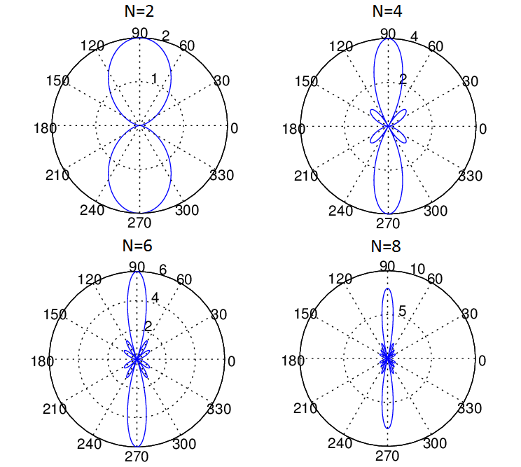
In the previous post we had discussed the fundamentals of a Uniform Linear Array (ULA). We had seen that as the number of array elements increases the Gain or Directivity of the array increases. We also discussed the Half Power Beam Width (HPBW) that can be approximated as 0.89×2/N radians. This is quite an accurate estimate provided that the number of array elements ‘N’ is sufficiently large.

Plane Wave Impinging Upon a ULA

But the max Gain is always in a direction perpendicular to the array. What if we want the array to have a high Gain in another direction such as 45 degrees. How can we achieve this? This has application in Radars where you want to search for a target by scanning over 360 degrees or in mobile communications where you want to send a signal to a particular user without causing interference to other users. One simple way is to physically rotate the antenna but that is not always a feasible solution.

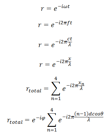
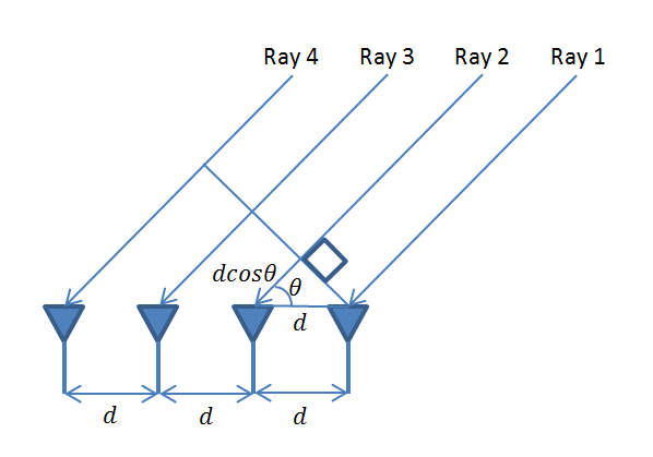
Going back to the basics remember that the Electric field pattern depends upon the constructive and destructive interference of incoming waves. If we have a vector (usually called the steering vector) that aligns the rays coming in from a particular direction we would get a high Gain in that direction. Similarly we can steer a null in a particular direction if we want to reject a particular signal. This we will discuss in a future post.

MATLAB CODE

%%%%%%%%%%%%%%%%%%%%%%%%%%%%%%%%%%%%
% BEAMFORMING USING A
% UNIFORM LINEAR ARRRAY
% COPYRIGHT RAYMAPS (C) 2018
%%%%%%%%%%%%%%%%%%%%%%%%%%%%%%%%%%%%

clear all
close all

f=1e9;
c=3e8;
l=c/f;
d=l/2;
no_elements=10;
phi=pi/6;

theta=0:pi/180:2*pi;
n=1:no_elements;
n=transpose(n);

X=exp(-i*(n-1)*2*pi*d*cos(theta)/l);
w=exp( i*(n-1)*2*pi*d*cos(phi)/l);
w=transpose(w);
r=w*X;

polar(theta,abs(r),'b')
title ('Gain of a Uniform Linear Array')

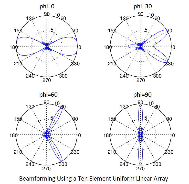
The figure below shows the Electric field pattern of a 10 element array steered towards 0, 30, 60 and 90 degrees respectively. We see that selectivity of the array is higher on the Broadside than on the Endfire. In my opinion this has to do with how the cosine function behaves from 0 to 90 degrees. The rate of change of cosine function is much faster around 90 degrees than at 0 degrees or 180 degrees. The slowly changing cosine in the latter case causes a wide response on the Endfire.

Beamforming Using a Ten Element Array

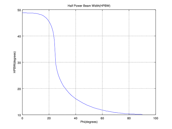
We did calculate the HPBW for a range of steering angles and found that it varied widely from as small as 10.17 degrees to as large as 48.62 degrees. This shows that simple Beamforming using a steering vector has its limitations. The detailed results along with a graph are shown below. It is seen that as the steering angle increases from about 20 degrees there is a sudden decrease in HPBW. For one degree increase of steering angle (phi) from 24 to 25 degrees there is decrease of approx 9 degrees in HPBW. We will investigate this further in future posts.

Case 1: phi = 0, HPBW = 48.62  deg
Case 2: phi = 30, HPBW = 21.69 deg
Case 3: phi = 60, HPBW = 11.75 deg
Case 4: phi = 90, HPBW = 10.17 deg

Half Power Beamwidth of a ULA
Half Power Beamwidth of a ULA as a function of Steering Angle (Phi)

For further visualization of the variation in antenna pattern as a function of the steering angle please have a look at this Interactive Graph. The parameters that can be varied include the angle of the beam, number of antenna elements and separation of the antenna elements. This is taken from an excellent online resource by the name of Geogebra. For further information on how you can use this tool for your own mathematical problems please do visit their website.

MY FIRST GEOGEBRA VISUALIZATION

Fundamentals of a Uniform Linear Array (ULA)

Introduction

A Uniform Linear Array (ULA) is a collection of sensor elements equally spaced along a straight line. The most common type of sensor is a dipole antenna that can transmit and receive Electromagnetic Waves over the air. Other types of sensors include acoustic sensors that may be used in air or under water. The requirements of a ULA are different for different applications but the most common requirement is to improve the Signal to Noise Ratio (SNR) and to improve its response (Gain) in a particular direction. The second property means that the array accepts a signal from a particular direction and rejects the signal from another direction just as required in Radar.

Excess Path Length

The graphical representation and the mathematical framework for the problem are shown below. It is assumed that Electromagnetic Waves (Rays) arrive at the array in the form of a plane wave. This means that there is a large distance between the transmitter and receiver (the receiver is in the far field of the transmitter). The array elements are separated by a distance ‘d’ which must be less than or equal to half the wavelength (similar to the concept of minimum sampling frequency in DSP). Now we can see that the second ray travels an excess distance dcos(θ). Similarly, the third and fourth rays travel an excess distance of 2dcos(θ) and 3dcos(θ) respectively. In array processing it is this excess distance between the arriving rays that is important, absolute distance from the source does not matter (unless you are interested in large scale effects such as path loss). This excess distance between the different rays determines if the signals are going to add constructively or destructively.

Plane Wave Impinging Upon a ULA
Plane Wave Impinging Upon a ULA (four elements)

Mathematical Model of a ULA

Mathematical Framework for ULA (four elements)

Simulation Methodology

Given below is the MATLAB code for the scenario shown in the figure above. We have considered two methods, one employing a ‘for-loop’ and another using matrix manipulation. The second method is usually preferred as it is much faster and also allows us to directly apply techniques from linear estimation theory. We have plotted the array pattern for four cases with N=2,4,6 and 8. It is seen that as the number of array elements increases the Gain (or Directivity) of the array increases. In the case shown below we have considered that the four received signals are added with equal weights (w=1), but these weights can be adjusted to get various beam patterns (weights are typically complex quantities adjusting both phase and amplitude  of the signal). This is typically called Beamforming and we will discuss this in a future post.

Matlab Code

FOR LOOP IMPLEMENTATION

%%%%%%%%%%%%%%%%%%%%%%%%%%%%%%%%%%%% 
% SIMPLE UNIFORM LINEAR ARRRAY
% WITH VARIABLE NUMBER OF ELEMENTS
% COPYRIGHT RAYMAPS (C) 2018
%%%%%%%%%%%%%%%%%%%%%%%%%%%%%%%%%%%%
clear all
close all
f=1e9;
c=3e8;
l=c/f;
d=l/2;
no_elements=4;
theta=0:pi/180:2*pi;
r=zeros(1,length(theta));
for n=1:no_elements
dx(n,:)=(n-1)*d*cos(theta);
r=r+exp(-i*2*pi*(dx(n,:)/l));
end
polar(theta,abs(r),'b')
title ('Gain of a Uniform Linear Array')

MATRIX IMPLEMENTATION

%%%%%%%%%%%%%%%%%%%%%%%%%%%%%%%%%%%% 
% SIMPLE UNIFORM LINEAR ARRRAY
% WITH VARIABLE NUMBER OF ELEMENTS
% MATRIX IMPLEMENTATION
% COPYRIGHT RAYMAPS (C) 2018
%%%%%%%%%%%%%%%%%%%%%%%%%%%%%%%%%%%%
clear all
close all
f=1e9;
c=3e8;
l=c/f;
d=l/2;
no_elements=4;
theta=0:pi/180:2*pi;
n=1:no_elements;
n=transpose(n);
A=(n-1)*(i*2*pi*d*cos(theta)/l);
X=exp(-A);
w=ones(1,no_elements);
r=w*X;
polar(theta,abs(r),'r')
title ('Gain of a Uniform Linear Array')

MATLAB Plot

Gain of a Uniform Linear Array with varying array length, N=2,4,6,8

Note: For a Uniform Linear Array with N elements and half wavelength inter-element spacing the Half Power Beam Width (HPBW) can be estimated as 1.78/N Radians [source]. For the four element case shown above the formula gave a HPBW of 25.49 degrees whereas our simulation yielded 26.20 degrees. For ten element case the formula gave a HPBW of 10.19 degrees whereas the simulation result was 10.20 degrees. Similarly the result for 20 elements is also quite accurate. So we can say that the formula does help us to get a ballpark estimate and gives progressively more accurate results as the number of elements is increased. For a general case where the inter-element spacing is not equal to half wavelength the formula is 0.89*(wavelength/total aperture length).

Lastly, for those who still do not know what Half Power Beam Width also known as 3dB Bandwidth means, it is the width of the main lobe in degrees 3dB down from the peak value of the radiation pattern.

Ibn al-Haytham to Maxwell: A Long Road

As the Chinese proverb says “The journey of a thousand miles begins with a single step”. The journey that started with Ibn al-Haytham experimenting with his Camera Obscura in the eleventh century was completed eight hundred years later by James Clerk Maxwell and Heinrich Hertz. While Maxwell laid down the mathematical framework that described the behavior of Electromagnetic waves, Hertz conclusively proved the existing of these invisible waves through his experiments. There were several scientists on the way that played a crucial part in development of this Electromagnetic theory such as Gauss, Faraday and Ampere. Then there were others such as Huygens, Fresnel and Young who worked on nature of light, which was not known to be an Electromagnetic wave at that time. Once the theory  of Electromagnetic wave propagation was in place there was rapid progress in many fields, particularly in wireless communications (wireless telegraph, radio, radar etc.).

Maxwell’s equations that were proposed in 1861 were initially quite circuitous and were not well accepted. But later on these equations were simplified into the form we now know by Oliver Heaviside. There are still two popular forms of the equations, the integral form and the differential form. We present the integral form of these equations in this article as it is more intuitive and is also easier to represent graphically. The differential form requires understanding of the concepts of divergence and curl and we skip it in this article. The main take away from these equations (presented below) is that a changing Electric field produces a Magnetic field and a changing Magnetic field produces an Electric field. Another important result is that magnetic monopoles do not exist (simply put a magnet, however small, always has a north and south pole).

Maxwell's Equations in Integral Form
Maxwell’s Equations in Integral Form

Note:

  1. The dot product with a line segment means that only that component of the field vector is effective that is along the line segment. On the other hand the dot product with a surface means that only that component is considered that is perpendicular to the surface (since the unit vector of a surface is perpendicular to the surface). It means that only those field components are considered that are going perpendicularly in or out of the surface.
  2. For more on history of Maxwell equations visit IEEE Spectrum  and for a detailed explanation of the various forms of the Maxwell’s equations visit this page.
  3. In modern Electromagnetic simulation software the differential form is preferred and the algorithm used is called Finite Difference Time Domain (FDTD). However, if the area of interest is quite large (with respect to the wavelength) then the FDTD method becomes prohibitively complex and another method known as Ray-Tracing is used. Please do check out the Ray-Tracing engine that we have developed. Ray-Tracing is becoming increasingly important in RF Planning of Telecom Networks.

Omar Khayyam’s Solution to Cubic Equations

Omar Khayyam was a Muslim mathematician and poet of the 11th and 12th centuries (1048-1131). His poetic works known as Rubaiyat of Omar Khayyam were translated from Persian to English and made popular by Edward Fitzgerald in the late nineteenth century. In the field of mathematics his most valuable contribution was the solution he presented to the cubic equations using geometrical methods. Some of this was adapted from earlier works by Greeks but his compilation of the various cases and their solutions was most complete.

Lets assume that the cubic equation also known as the third degree equation (highest power of the unknown variable) is of the form:

x3+a2x=b

Khayyam’s method consisted of constructing a parabola with equation x2=ay and a circle with center (b/2a2,0) and radius b/2a2. Then the x-coordinate of the intersection of the circle and the parabola gives the solution to the cubic equation. The root found by this method is the real and positive root since the length of a line segment cannot be negative or imaginary. These cases (negative and imaginary roots) were not discussed by Khayyam and were worked out much later by other mathematicians. The MATLAB code for this geometrical construction is given below.

%%%%%%%%%%%%%%%%%%%%%%%%%%%%%%%%
% Omar Khayyams Method to Find  
% the Roots of a Cubic Equation 
%
% Copyright RAYmaps 2017 (YA)
%%%%%%%%%%%%%%%%%%%%%%%%%%%%%%%%
clear all
close all

% Plot the parabola
a =5;
x =-5:0.01:5;
y =(x.^2)/a;
plot(x,y,'linewidth',4);
hold on

% Plot the circle
b =100;
d =b/(a.^2);
r =d/2;
t =0:pi/180:2*pi;
plot(r+r*cos(t), r*sin(t),'r', 'linewidth', 4);
hold off
axis([-5 5 -5 5], "square")
grid on
title('Khayyams Method to Solve Cubic Equations')
xlabel('x')
ylabel('y')

Omar Khayyam's Method for Solving Cubic Equations

Omar Khayyam’s Method for Solving Cubic Equations

Notes:

  1. For more on origins of geometrical methods see the following post on Al-Khwarizmi.
  2. For an interactive tool to understand the method of Omar Khayyam visit the following page.
  3. For a proof of validity of Khayyam’s method see the following page on Cornell website or see selected abstract below. Please note slightly different form of the equation where the term a2 has been replaced by a. This is just a constant term and either form works.

Proof of Khayyam's Method from Cornell