We have been using a wireless signal model in our simulations without going into the details of noise calibration for simulation. In this article we discuss this. Lets assume the received signal is given as

r(t)=s(t)+n(t)

where r(t) is the received signal s(t) is the transmitted signal and n(t) is the Additive White Gaussian Noise (AWGN). Channel fading is ignored at the moment. Signal to noise ratio for simulation of digital communication systems is given as

ρ=Eb/No (1)

Where Eb is the energy per bit and No is the noise Power Spectral Density (PSD). We also know that for the case of Additive White Gaussian Noise the noise power is given as [Tranter]

σ^2=(No/2)*fs

No=2*(σ^2)/fs

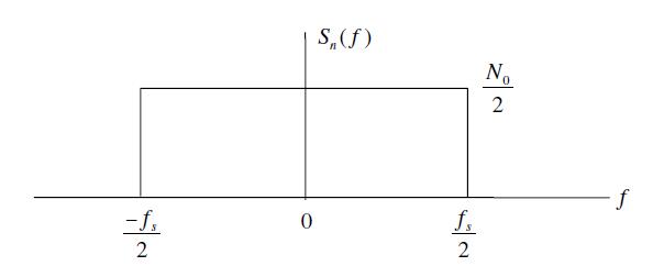Where σ is the standard deviation of noise and fs is the sampling frequency.  Substituting in equation 1 we get

ρ=Eb/No=Eb/(2*σ^2/fs )

Eb/No=(Eb*fs)/(2*σ^2)

σ^2=(Eb*fs)/(2*Eb/No )

σ=√((Eb*fs)/(2*Eb/No ))

If the energy per bit and the sampling frequency is set to 1 the above equation reduces to

σ=√(1/(2*Eb/No ))

The simulation software can thus calculate the noise standard deviation (or variance) for each value of Eb/No in the simulation cycle. The following piece of MATLAB code generates AWGN with the required power and adds it to the transmitted signal.

s=sign(rand-0.5);      % Generate a symbol
sigma=1/sqrt(2*EbNo);  % Calculate noise standard deviation
n=sigma*randn;         % Generate AWGN with the required std dev 
r=s+n;                 % Add noise to the signal

How can we assume that energy per bit and sampling frequency is equal to one and are we breaking some discrete time signal processing rule here. This will be discussed in a later post.