We have previously discussed the Bit Error Rate of M-QAM in Rayleigh Fading using Monte Carlo Simulation. We now turn our attention to calculation of Bit Error Rate (BER) of M-QAM in Rayleigh fading using analytical techniques. In particular we look at the method used in MATLAB function berfading.m. In this function the BER of 4-QAM, 16-QAM and 64-QAM is calculated from series expressions having 1, 3 and 5 terms respectively. These are given below (M is the constellation size and must be a power of 2).
if (M == 4)
     ber = 1/2 * ( 1 - sqrt(gamma_c/k./(1+gamma_c/k)) );
elseif (M == 16)
     ber = 3/8 * ( 1 - sqrt(2/5*gamma_c/k./(1+2/5*gamma_c/k)) ) ...
     + 1/4 * ( 1 - sqrt(18/5*gamma_c/k./(1+18/5*gamma_c/k)) ) ...
     - 1/8 * ( 1 - sqrt(10*gamma_c/k./(1+10*gamma_c/k)) );
elseif (M == 64)
     ber = 7/24 * ( 1 - sqrt(1/7*gamma_c/k./(1+1/7*gamma_c/k)) ) ...
     + 1/4 * ( 1 - sqrt(9/7*gamma_c/k./(1+9/7*gamma_c/k)) ) ...
     - 1/24 * ( 1 - sqrt(25/7*gamma_c/k./(1+25/7*gamma_c/k)) ) ...
     + 1/24 * ( 1 - sqrt(81/7*gamma_c/k./(1+81/7*gamma_c/k)) ) ...
     - 1/24 * ( 1 - sqrt(169/7*gamma_c/k./(1+169/7*gamma_c/k)) );
Although using these expressions we get very accurate BER but it is not that simple to calculate (the expressions become even more complicated for higher constellation sizes such as 256-QAM). Therefore we try to simplify these expressions by using only the first term in each expression. To our surprise the results match quite well with the results using the exact formulae. There is very minor difference at low signal to noise ratios but that can be easily bargained for the ease of calculation.
So here is our program for calculating the BER using the approximate method.
%%%%%%%%%%%%%%%%%%%%%%%%%%%%%%%%%%%%%%%%%%%%%%%%%%%%%%%%%%%%%%%%%%%%%%%%%%%
% FUNCTION TO CALCULATE THE BER OF M-QAM IN RAYLEIGH FADING
% M: Input, Constellation Size
% EbNo: Input, Energy Per Bit to Noise Power Spectral Density
% ber: Output, Bit Error Rate
%%%%%%%%%%%%%%%%%%%%%%%%%%%%%%%%%%%%%%%%%%%%%%%%%%%%%%%%%%%%%%%%%%%%%%%%%%%
function [ber]= BER_QAM_fading (M, EbNo)

k=log2(M);
EbNoLin=10.^(EbNo/10);
gamma_c=EbNoLin*k;

if M==4
    %4-QAM
    ber = 1/2 * ( 1 - sqrt(gamma_c/k./(1+gamma_c/k)) );
elseif M==16
    %16-QAM
    ber = 3/8 * ( 1 - sqrt(2/5*gamma_c/k./(1+2/5*gamma_c/k)) );
elseif M==64
    %64-QAM
    ber = 7/24 * ( 1 - sqrt(1/7*gamma_c/k./(1+1/7*gamma_c/k)) );
else
    %Warning
    warning('M=4,16,64')
    ber=zeros(1,length(EbNo));
end

semilogy(EbNo,ber,'o-')
xlabel('EbNo(dB)')
ylabel('BER')
axis([0 24 0.001 1])
grid on

return
%%%%%%%%%%%%%%%%%%%%%%%%%%%%%%%%%%%%%%%%%%%%%%%%%%%%%%%%%%%%%%%%%%%%%%%%%%%
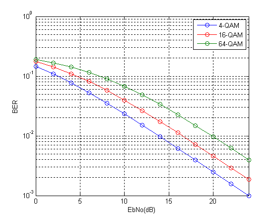
So we see that the results match quite well with the results previously obtained through simulation. We will next tackle the problem of simplifying the expression for higher order modulations such as 256-QAM in both Rayleigh and Ricean channels.